Multivariate

A function expresses the idea that one quantity (the argument of the function) completely determines another quantity (the value).

Interpolation is a method of constructing new data points within the range of a discrete set of known data points.

Multivariate interpolation, nearest-neighbor, bilinear, multilinear, bicubic, multicubic

View versions (2)

Definition

Multivariate interpolation is an area of data fitting which, as opposed to univariate interpolation which fitted two-dimensional data points, finds the surface that provides an exact fit to a series of multidimensional data points. It is called multivariate since the data points are supposed to be sampled from a function of several variables.

Formally speaking, consider a series of $N$ distinct $(d + 1)$ - dimensional data points $(x_1, y_1)$ , $(x_2, y_2), \ldots, (x_N, y_N)$ , where $x_i := (x_i^1, x_i^2, \ldots, x_i^d)$ is a vector, for each $i = 1, 2, \ldots, N$ . By interpolating these data points we mean finding a function $f : \mathbb{R}^d \to \mathbb{R}$ such that:

$f(x_1) = y_1, \quad f(x_2) = y_2, \quad \ldots \quad f(x_N) = y_N.$

We will start by describing the most straightforward multivariate interpolation methods, to the more advanced. We start with the description of the method in 3D, and then explain how this generalizes to multidimensional space.

Nearest-neighbor interpolation

This type of interpolation basically assigns to any point $P(x, y)$ in the plane, the value of the closest data point to $P$ . Formally, given a series of data points $(x_i, y_i, z_i)$ , for $i = 1, 2, \ldots, N$ , the corresponding nearest-neighbor interpolation function is given by

$f(x, y) = f(x^*, y^*)$

where $(x^*, y^*)$ is the closest data point to $(x, y)$ in the sense of Euclidean distance. In other words, $(x^*, y^*)$ minimizes the following objective function

$\delta(x_i, y_i) := \sqrt{(x - x_i)^2 + (y - y_i)^2}$

where $i = 1, 2, \ldots, N$ . The image below shows how nearest-neighbor interpolation is applied to a series of data points in the box $[0, 3] \times [0, 3]$ .

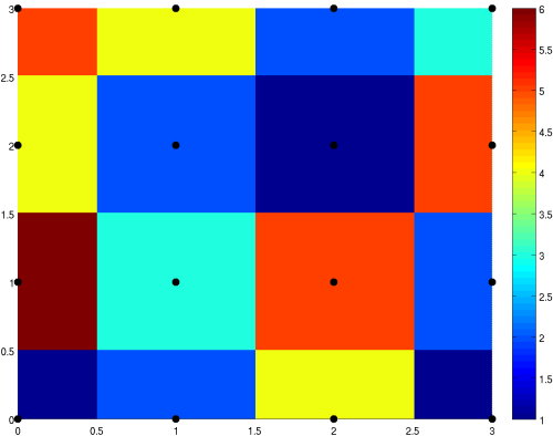
In general d-dimensional space, nearest-neighbor interpolation assigns to some point $P(x_1, x_2, \ldots, x_d)$ the value of the closest data point $P(x_1^*, x_2^*, \ldots, x_d^*)$ to $P$ , i.e. the one which minimizes the objective function

$\delta(x_i^1, x_i^2, \ldots, x_i^d) := \sqrt{(x_1 - x_i^1)^2 + (x_2 - x_i^2)^2 + \ldots + (x_d - x_i^d)^2}$

for all $i = 1, 2, \ldots, N$ , where $(x_i^1, x_i^2, \ldots, x_i^d, y_i)$ are the given data points.

Bilinear interpolation

This is a generalization of linear interpolation, from 2D to 3D data points. It is assumed that the given data points are distributed along an uniform grid, as are the points $Q_{11}$ , $Q_{12}$ , $Q_{21}$ and $Q_{22}$ in the image below.

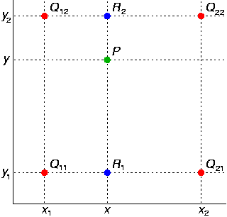
The aim is to estimate the value of the function $f(x, y)$ (from which the data points have been sampled) at point $P(x, y)$ in the above graph. In order to do this, let us define two auxiliary functions $f_1, f_2 : \mathbb{R} \to \mathbb{R}$ through

$f_1(x) = f(x, y_1), \qquad f_2(x) = f(x, y_2)$

where the coordinates of $Q_{ij}$ are $(x_i, y_j)$ and $z_{ij} := f(Q_{ij})$ .

The next thing is to do linear interpolation on the two-dimensional data points $(x_1, z_{11})$ , $(x_2, z_{21})$ and $(x_1, z_{12})$ , $(x_2, z_{22})$ correspondingly. In other words, the linear interpolation functions $f_1$ , $f_2$ can be given by:

$f_1(x) = \frac{x_2 - x}{x_2 - x_1} z_{11} + \frac{x - x_1}{x_2 - x_1} z_{21}\ \ , \qquad f_2(x) = \frac{x_2 - x}{x_2 - x_1} z_{12} + \frac{x - x_1}{x_2 - x_1} z_{22}$

All that is left is to do linear interpolation on the two-dimensional data points $(y_1, f_1(x))$ and $(y_2, f_2(x))$ , providing the desired formula for the interpolation function $f(x, y)$

$f(x, y) = \frac{y_2 - y}{y_2 - y_1} f_1(x) + \frac{y - y_1}{y_2 - y_1} f_2(x)$

which, with the above notations, can be written:

$\begin{array}{rl} f(x, y) \approx \frac{\displaystyle 1}{\displaystyle (x_2 - x_1)(y_2 - y_1)} & \left[ z_{11} (x_2 - x)(y_2 - y) + z_{21} (x - x_1)(y_2 - y) + \right. \\ & \left. + z_{12} (x_2 - x)(y - y_1) + z_{22} (x - x_1)(y - y_1) \right] \end{array}$

This solves the problem of doing bilinear interpolation for a set of 4 three-dimensional points. If there are more than 4 points (they should however be a multiple of 2), then we repeat the above algorithm for each cell. The interpolation function over the entire domain is then defined in a piecewise manner on each cell, through the corresponding bilinear interpolation function for that cell.

The image below shows the values obtained by applying linear interpolation on the same series of data points as in the previous graph.

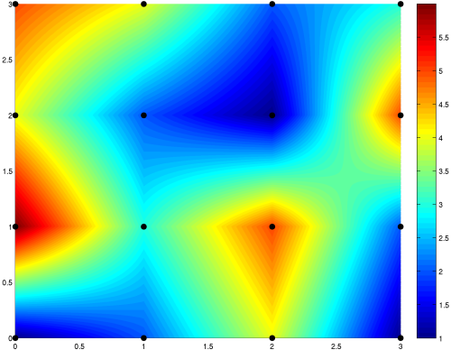
Using the same reasoning as above, we are able to generalize linear interpolation from some d-dimensional space to (d + 1)-dimensional space, in a recursive manner, giving birth to multilinear interpolation. The concept of uniform grid also generalizes to multidimensional space, as seen in the article: http://en.wikipedia.org/wiki/Honeycomb_(geometry) .

Bicubic Interpolation

Without loss of generality, consider that we are given the values of the points $(0, 0)$ , $(0, 1)$ , $(1, 0)$ and $(1, 1)$ , i.e. the corners of the unit box $[0, 1] \times [0, 1]$ . Our aim is to find a bicubic function $p(x, y)$ of the form

$p(x, y) = \sum_{i = 0}^3 \sum_{j = 0}^3 a_{ij} x^i y^j$

that provides an exact fit to the given data points. In order to determine $p$ , we need to determine its coefficients $\displaystyle a_{ij}$ . This is only possible if the values of the partial derivatives $\displaystyle \frac{\partial f}{\partial x}$ , $\displaystyle \frac{\partial f}{\partial x}$ and $\displaystyle \frac{\partial^2 f}{\partial x \partial y}$ are know at each corner of the unit box.

In this case, by writing the set of linear equations

$f(T) = p(T), \quad \frac{\partial f}{\partial x}(T) = \frac{\partial p}{\partial x}(T), \quad \frac{\partial f}{\partial y}(T) = \frac{\partial p}{\partial y}(T), \quad \frac{\partial^2 f}{\partial x \partial y}(T) = \frac{\partial^2 p}{\partial x \partial y}(T),$

for all $T \in \{(0, 0), (0, 1), (1, 0), (1, 1)\}$ , we are able to find the coefficients $\displaystyle a_{ij}$ and completely determine the bicubic interpolation function $p$ . As in the case of bilinear interpolation, if there are more than 4 points, then we repeat the above algorithm for each cell. The bicubic interpolation function over the entire domain is then defined in a piecewise fashion on each cell, through the corresponding bicubic interpolation function for that cell. It is also required that all the partial derivatives match on the common boundary of each pair of cells.

The following image shows the values obtained using bicubic interpolation on the same series of data points as in the previous graphs.

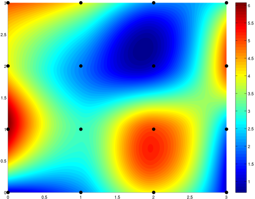
Generally, using bicubic instead of bilinear or nearest-neighbor interpolation results in smoother approximations and thus is more advantageous in image restoration techniques.

When generalizing this method to multidimensional space, the function $p$ will be of the form

$p(x_1, x_2, \ldots, x_d) := \sum_{i_1 = 0}^d \sum_{i_2 = 0}^d \cdots \sum_{i_d = 0}^3 a_{i_1 i_2 \ldots i_d} x_1^{i_1} x_2^{i_2} \ldots x_d^{i_d}$

and of course several other partial derivatives may come into play. The resulting system, although large, will still be linear and will allow us to find the coefficients $a_{i_1 i_2 \ldots i_d}$ of the cubic interpolation function $p$ . This method is also called multicubic interpolation.

Author Lucian Bentea

Multivariate

Definition

Nearest-neighbor interpolation

Bilinear interpolation

Bicubic Interpolation

References