
Linear
Linearly interpolates a given set of points.
Interface
#include <codecogs/maths/approximation/interpolation/linear.h>
using namespace Maths::Approximation::Interpolation;
Overview
Linear interpolation is a process employed in mathematics, and numerous applications thereof including computer graphics. It is a very simple form of interpolation. In numerical analysis a linear interpolation of certain points that are in reality values of some function f is typically used to approximate the function f. Linear interpolation can be regarded as a trivial example of polynomial interpolation. The error of this approximation is defined as
where p denotes the linear interpolation polynomial defined as follows
It can be proven using Rolle's theorem that if f has two continuous derivatives, the error is bounded by
As you see, the approximation between two points on a given function gets worse with the second derivative of the function that is approximated. This is intuitively correct as well: the "curvier" the function is, the worse is the approximations made with simple linear interpolation.
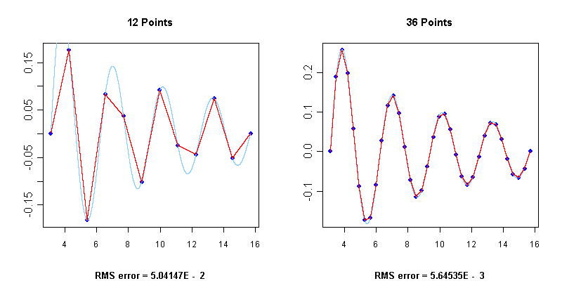
Below you will find the interpolation graphs for a set of points obtained by evaluating the function , displayed in light blue, at particular abscissas. The linear interpolating function, displayed in red, has been calculated using this class. In the first graph there had been chosen a number of 12 points, while in the second 36 points were considered. You may notice the root mean squared error in each of the cases.
References
Wikipedia, http://en.wikipedia.org/wiki/Linear_interpolation
Example 1
The following example displays 20 interpolated values (you may change this amount through the N_out variable) for the given function with abscissas equally spaced in the
interval. The X and Y coordinate arrays are initialized by evaluating this function for N = 12 points equally spaced in the domain from
to
.
#include <codecogs/maths/approximation/interpolation/linear.h>

#include <cmath>
#include <iostream>
#include <iomanip>
using namespace std;

#define PI  3.1415
#define N   12

int main()
{
    // Declare and initialize two arrays to hold the coordinates of the initial data points
    double x[N], y[N];

    // Generate the points
    double xx = PI, step = 4 * PI / (N - 1);
    for (int i = 0; i < N; ++i, xx += step) {
        x[i] = xx;
        y[i] = sin(2 * xx) / xx;
    }

    // Initialize the linear interpolation routine with known data points
    Maths::Interpolation::Linear A(N, x, y);

    // Interrogate linear fitting curve to find interpolated values
    int N_out = 20;
    xx = PI, step = (3 * PI) / (N_out - 1);
    for (int i = 0; i < N_out; ++i, xx += step) {
        cout << "x = " << setw(7) << xx << "  y = ";
        cout << setw(13) << A.getValue(xx) << endl;
	}
    return 0;
}
Output:
x =  3.1415  y = -5.89868e-005
x = 3.63753  y =     0.0765858
x = 4.13355  y =      0.153231
x = 4.62958  y =     0.0678533
x = 5.12561  y =    -0.0879685
x = 5.62163  y =     -0.137135
x = 6.11766  y =     -0.022215
x = 6.61368  y =     0.0804548
x = 7.10971  y =      0.060627
x = 7.60574  y =     0.0407992
x = 8.10176  y =    -0.0110834
x = 8.59779  y =    -0.0715961
x = 9.09382  y =    -0.0619804
x = 9.58984  y =     0.0221467
x = 10.0859  y =      0.081803
x = 10.5819  y =     0.0313408
x = 11.0779  y =    -0.0191214
x = 11.5739  y =    -0.0324255
x =   12.07  y =    -0.0406044
x =  12.566  y =    -0.0146181
See Also
Also consider the regression methods: Discrete, Forsythe, Orthogonal, Stiefel
Members of Linear
CLASS METHOD
Linear
Initializes the necessary data for following evaluations of the fitting lines.
Parameters
CLASS METHOD
Linear
CLASS METHOD
getValue
Returns the approximated ordinate at the given abscissa.
Parameters
This function is not designed to provide extrapolation points, thus you need to keep the value of x in the interval from X[0] to X[N - 1].
CLASS METHOD
Linear_once
This function implements the Linear class for one off calculations, thereby avoid the need to instantiate the Linear class yourself.
Example 1
The following graph is constructed from interpolating the following values:
x = 1  y = 0.22
x = 2  y = 0.04
x = 3  y = -0.13
x = 4  y = -0.17
x = 5  y = -0.04
x = 6  y = 0.09
x = 7  y = 0.11
\graph N=7 x="1 2 3 4 5 6 7" y="0.22 0.04 -0.13 -0.17 -0.04 0.09 0.11" a=1:7 .input