Engineering › Materials ›

Shear Force and Bending Moment

An introduction to Shear Force and Bending Moments in Beams.

View other versions (5)

Contents

Introduction
Shearing Force
Bending Moments
Types Of Load
Types Of Support
The Relationship Between W, F, M.
Concentrated Loads
Uniformly Distributed Loads
Combined Loads.
Varying Distributed Loads.
Graphical Solutions
Appendix
Page Comments

Introduction

MISSING IMAGE!

23573/0001.jpg cannot be found in /users/23573/0001.jpg. Please contact the submission author.

Shear Forces occurs when two parallel forces act out of alignment with each other. For example, in a large boiler made from sections of sheet metal plate riveted together, there is an equal and opposite force exerted on the rivets, owing to the expansion and contraction of the plates.

Bending Moments are rotational forces within the beam that cause bending. At any point within a beam, the Bending Moment is the sum of: each external force multiplied by the distance that is perpendicular to the direction of the force.

Shearing Force

MISSING IMAGE!

23287/SF-and-BM-0001.png cannot be found in /users/23287/SF-and-BM-0001.png. Please contact the submission author.

The shearing force (SF) at any section of a beam represents the tendency for the portion of the beam on one side of the section to slide or shear laterally relative to the other portion.

The diagram shows a beam carrying loads $\inline \displaystyle W_1\;\;, W_2\;\;and\;\;W_3$ . It is simply supported at two points where the reactions are $\inline \displaystyle R_1\;\;\;and\;\;\;R_2$ . Assume that the beam is divided into two parts by a section XX. The resultant of the loads and reaction acting on the left of AA is F vertically upwards, and since the whole beam is in equilibrium, the resultant force to the right of AA must be F downwards. F is called the Shearing Force at the section AA. It may be defined as follows:-

The shearing force at any section of a beam is the algebraic sum of the lateral components of the forces acting on either side of the section.

Where forces are neither in the lateral or axial direction they must be resolved in the usual way and only the lateral components are used to calculate the shear force.

Bending Moments

MISSING IMAGE!

23287/SF-and-BM-0002.png cannot be found in /users/23287/SF-and-BM-0002.png. Please contact the submission author.

In a similar manner it can be seen that if the Bending moments (BM) of the forces to the left of AA are clockwise, then the bending moment of the forces to the right of AA must be anticlockwise.

Bending Moment at AA is defined as the algebraic sum of the moments about the section of all forces acting on either side of the section.

Bending moments are considered positive when the moment on the left portion is clockwise and on the right anticlockwise. This is referred to as a sagging bending moment as it tends to make the beam concave upwards at AA. A negative bending moment is termed hogging.

Types Of Load

A beam is normally horizontal and the loads vertical. Other cases which occur are considered to be exceptions.

A Concentrated load is one which can be considered to act at a point, although in practice it must be distributed over a small area.

A Distributed load is one which is spread in some manner over the length, or a significant length, of the beam. It is usually quoted at a weight per unit length of beam. It may either be uniform or vary from point to point.

Types Of Support

A Simple or free support is one on which the beam is rested and which exerts a reaction on the beam. It is normal to assume that the reaction acts at a point, although it may in fact act act over a short length of beam.

MISSING IMAGE!

23287/SF-and-BM-0005.png cannot be found in /users/23287/SF-and-BM-0005.png. Please contact the submission author.

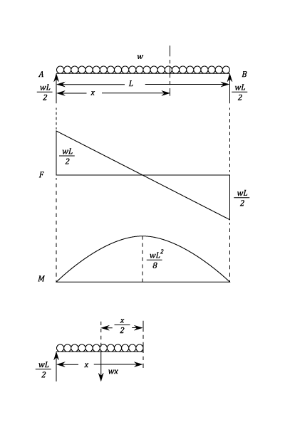
A Built-in or encastre' support is frequently met . The effect is to fix the direction of the beam at the support. In order to do this the support must exert a "fixing" moment M and a reaction R on the beam. A beam which is fixed at one end in this way is called a Cantilever. If both ends are fixed in this way the reactions are not statically determinate.

In practice, it is not usually possible to obtain perfect fixing and the fixing moment applied will be related to the angular movement of the support. When in doubt about the rigidity, it is safer to assume that the beam is freely supported.

The Relationship Between W, F, M.

In the following diagram $\inline \displaystyle \delta x$ is the length of a small slice of a loaded beam at a distance x from the origin O

MISSING IMAGE!

23287/SF-and-BM-0004.png cannot be found in /users/23287/SF-and-BM-0004.png. Please contact the submission author.

Let the shearing force at the section x be F and at $\inline \displaystyle x = \delta x\;\;be\;\;F + \delta F$ . Similarly, the bending moment is M at x, and $\inline \displaystyle M + \delta M\;\;\;at\;\;\;x + \delta x$ . If w is the mean rate of loading of the length $\inline \displaystyle \delta x$ , then the total load is $\inline \displaystyle w\delta x$ , acting approximately (exactly if uniformly distributed) through the centre C. The element must be in equilibrium under the action of these forces and couples and the following equations can be obtained:-

Taking Moments about C:

$M + F.\frac{\delta x}{2} + (F + \delta F)\;\frac{\delta x}{2} = M + \delta M$

(2)

Neglecting the product $\inline \displaystyle \delta F.\delta x$ in the limit:

$F = \frac{dM}{dx}$

(3)

Resolving vertically:

$w\delta x + F + \delta F = F$

(4)

$Or\;\;\;\;\;\;\;w = -\frac{dF}{dx}$

(5)

$= -\frac{d^2M}{dx^2}\;\;\;\;\;from\;equation\;(2)$

(6)

From equation (2) it can be seen that if M is varying continuously, zero shearing force corresponds to either maximum or minimum bending moment. It can be seen from the examples that "peaks" in the bending moment diagram frequently occur at concentrated loads or reactions, and these are not given by $\inline \displaystyle F = \frac{dM}{dx} = 0$ ; although they may in fact represent the greatest bending moment on the beam. Consequently, it is not always sufficient to investigate the points of zero shearing force when determining the maximum bending moment.

At a point on the beam where the type of bending is changing from sagging to hogging, the bending moment must be zero, and this is called a point of inflection or contraflexure.

By integrating equation (2) between the x = a and x = b then:

$M_b - M_a = \int_{a}^{b}F\,dx$

(7)

Which shows that the increase in bending moment between two sections is the area under the shearing force diagram.

Similarly integrating equation (4)

$F_a - F_b = \int_{a}^{b}w\,dx$

(8)

equals the area under the load distribution diagram.

Integrating equation (5) gives:

$M_a - M_b = \int \int_{a}^{b}w\,dx.dx$

(9)

These relations can be very valuable when the rate of loading cannot be expressed in an algebraic form as they provide a means of graphical solution.

Concentrated Loads

Example:

[imperial]

Example - Example 1

Problem

A Cantilever of length l carries a concentrated load W at its free end. Draw the Shear Force (SF) and Bending Moment (BM) diagrams.

Workings

Consider the forces to the left of a section at a distance x from the free end.

Then F = - W and is constant along the whole cantilever i.e. for all values of x

Taking Moments about the section gives M = - W x so that the maximum Bending Moment occurs when x = l i.e. at the fixed end.

$\hat{M} = W\,l\;\;\;(Hogging)$

(1)

From equilibrium considerations it can be seen that the fixing moment applied at the built in end is WL and the reaction is W. Hence the SF and BM diagrams are as follows:

The following general conclusions can be drawn when only concentrated loads and reactions are involved.

The shearing force suffers sudden changes when passing through a load point. The change is equal to the load.
The bending Moment diagram is a series of straight lines between loads. The slope of the lines is equal to the shearing force between the loading points.

Uniformly Distributed Loads

Example:

[imperial]

Example - Example 3

Problem

Draw the SF and BM diagrams for a Simply supported beam of length l carrying a uniformly distributed load w per unit length which occurs across the whole Beam.

Workings

The Total Load carried is wl and by symmetry the reactions at both end supports are each wl/2

If x is the distance of the section measured from the left-hand support then:

$F = \frac{wl}{2} - wx = w\left(\frac{l}{2} - x \right)$

(2)

This give a straight line graph equal to the rate of loading. The end values of Shearing Force are $\displaystyle \pm \frac{w\,l}{2}$

The Bending Moment at the section is found by assuming that the distributed load acts through its center of gravity which is x/2 from the section.

$Hence\;\;\;\;\;\;M = \left(\frac{w\,l}{2} \right)x - (wx)\;\frac{x}{2}$

(3)

$= \left(\frac{wl}{2} \right)\left(l - x \right)$

(4)

This is a parabolic curve having a value of zero at each end. The maximum is at the center and corresponds to zero shear force.

From Equation (2)

$\hat{M} = \left(\frac{w\,l}{4} \right)\left(l - \frac{l}{2} \right)$

(5)

Putting x = l/2

$\hat{M} = \frac{w\,l^2}{8}$

(6)

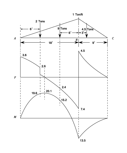
Combined Loads.

Example:

[imperial]

Example - Example 4

Problem

A Beam 25 ft. long is supported at A and B and is loaded as shown. Sketch the SF and BM diagrams and find (a) the position and magnitude of the maximum Bending Moment and (b) the position of the point of contra flexure.

Workings

Taking Moments about B

$20\,R_a = 10\times15 + 2\times5 - 3\times5$

(7)

(The distributed load is taken as acting at its centre of gravity.)

$\therefore\;\;\;\;\;\;R_a = 7.25\;tons$

(8)

$\therefore\;\;\;\;\;\;R_b = Total\; Load - R_a = 10 + 2 + 3 - 7.25 = 7.75\;tons$

(9)

The Shearing Force

Starting at A F = 7.25. As the section moves away from A F decreases at a uniform rate of w per unit length ( i.e. f =

7.25 - wx) and reaches a value of - 2.75 at E. Between E and D, F is constant ( There is no load on Ed) and at D it

suffers a sudden decrease of 2 tons ( the load at D) . Similarly there is an increase at B of 7.75 tons ( the reaction at

B). This results in a value of F = 3 tons at B which remains constant between B and C. Note this value agrees with the load at C.

Bending Moment From A to E:

$M = R_a\,x - \frac{w\,x^2}{2} = 7.25\,x - \frac{x^2}{2}\;\;\;\;since\;\;\;\;(x = 1)$

(10)

This is a parabola which can be sketched by taking several values of x. Beyond E the value of x for the distributed load

remains constant at 5 ft. from A

Between E and D

$M = 7.25\,x - 10(X - 5)\;= - 2.75x + 50$

(11)

This produces a straight line between E and D. Similar equations apply for sections DB and BC. However it is only

necessary to evaluate M at the points D and B since M is zero at C. The diagram consists in straight lines between these

values.

At D

$M = -2.75\times15 + 50 = 8.75\;\;tons-ft.$

(12)

At B

$M = -\,3\times5 = -\,15\;\;\;tons-ft.$

(13)

This last value was calculated for the portion BC

We were required to find the position and magnitude of the maximum BM. This occurs where the shearing force is zero.

i.e.at 7.25 ft. from A

$\therefore\;\;\;\;\;\;\hat{M} = 7.25\times7.25 - \frac{7.25^2}{2} = 26.28\;\;tons\,-\,ft.$

(14)

The point of contraflexure occurs when the bending moment is zero and this is between D and B at:

$\left(\frac{15}{15 + 8.75} \right)\times5 = 3.16\;\;ft.\;from\;B$

(15)

Varying Distributed Loads.

Example:

[imperial]

Example - Example 7

Problem

A Beam ABC, 27 ft. long, is simply supported at A and B 18 ft. across and carries a load of 2 tons at 6 ft. from A together with a distributed load whose intensity varies in linear fashion from zero at A and C to 1ton/ft. at B.

Workings

Draw the Shear Force and Bending Moment diagrams and calculate the position and magnitude of the maximum B.M. (U.L.)

The Total Load on the beam ( i.e. the load plus the mean rate of loading of 1/2 tons/ft) is given by: $Load = 2 + \frac{1}{2}\times27 = 15.5\,tons$

The Total distribute load on $\displaystyle AB = \frac{1}{2}\times18 = 9\;\;tons$ and on $\displaystyle BC = \frac{1}{2}\times9 = 4.5\;\;tons$ each of which act through their centres of gravity. These are $\displaystyle \frac{2}{3}\times 18 = 12\;\;ft.$ from A and $\displaystyle \frac{2}{3}\times 9 = 6\;\;ft.$ from C in the other case.

(Note. These are the centroids of the triangles which represent the load distribution)

Taking Moments about B

$R_1 = \left(\frac{2\times12 + 9\times6\;-4.5\times3}{18} \right) = 3.6\;\;tons$

(16)

$\therefore\;\;\;\;\;R_2 = 2 + 9 + 4.5 - 3.6 = 11.9\;\;tons$

(17)

At a distance x (<18)from A the loading is x/18 tons/ft.. The Total distributed load on this length is:

$(Mean\;rate\;of\;loading)\times x = \frac{1}{2}\left(\frac{x}{18} \right)\;x = \frac{x^2}{36}\;\;tons$

(18)

The centre of gravity of this load is $\displaystyle \frac{2}{3}\;x$ from A. For 0<x<6

$F = 3.6 - \frac{x^2}{36}$

(19)

At x = 6 ft.

$F = 2.6\;\;tons$

(20)

$M = 3.6\,x - \left(\frac{x^2}{36} \right)\times \frac{x}{3} = 3.6\,x - \frac{x^3}{108}$

(21)

At x = 6 ft.

$M = 19.6\;\;tons-ft.$

(22)

6< x <18

$f = 3.6 - 2 - \frac{x^2}{36}$

(23)

$At\;x = 12\;\;ft.\;\;\;\;\;\;\;\;F\;= - 2.4\;\;tons$

(24)

$At\;x = 18\;\;ft.\;\;\;\;\;\;\;\;F\;= - 7.4\;\;tons$

(25)

$F = 0\;\;\;\;when\;\;\;\;x = 6\;\sqrt{1.6} = 7.58\;ft.$

(26)

$M = 3.6x - 2(x - 6) - \frac{x^3}{108} = 1.6x + 12 - \frac{x^3}{108}$

(27)

$At\;x = 12\;\;ft\;\;\;\;\;\;\;\;M = 15.2\;\;tons-ft.$

(28)

$At\;x = 12\;\;ft\;\;\;\;\;\;\;\;M\;= - 13.5\;\;tons-ft.$

(29)

The maximum Bending Moment occurs at zero s earing force 1.e.x = 7.58 ft.

$\therefore\;\;\;\;\;\hat{M} = 20.1\;\;tons-ft.$

(30)

The section BC can be more easily calculated by using a variable X measured from C. Then by a similar argument:-

$F = \frac{1}{2}\left(\frac{X}{9} \right)X = \frac{X^2}{18}\;\;tons$

(31)

$At\;\;\;X = 9\;\;ft.\;\;\;\;\;\;\;\;F = 4.5\;\;tons.$

(32)

$M\;= - \frac{1}{2}\left(\frac{X}{9} \right)X\left(\frac{X}{3} \right)\;=\[-\frac{X^3}{54}\;\;ton-ft.$

(33)

$At\;\;\;X = 9\;\;ft.\;\;\;\;\;\;\;\;\;\;=- 13.5\;\;tons-ft.$

(34)

The complete diagrams are shown. It can e seen that for a uniformly varying distributed load, the Shearing Force diagram consists of a series of parabolic curves and the Bending Moment diagram is made up of "cubic" discontinuities occurring at concentrated loads or reactions. It has been shown that Shearing Forces can be obtained by integrating the loading function and Bending Moment by integrating the Shearing Force, from which it follows that the curves produced will be of a successively "higher order" in x ( See equations (6) and(7))

Graphical Solutions

Note This method may appear complicated but whilst the proof and explanation is fairly detailed, the application is simple and straight forward.

Earlier it was shown that the change of Bending Moment is given by the double Integral of the rate of loading. This integration can be carried out by means of a funicular polygon. See diagram.

Suppose that the loads carried on a simply supported beam are $\inline \displaystyle W_1, W_2, W_3, and W_4 , and that R_1\;and\;R_2$ are the reactions at the supports. Letter the spaces between the loads and reactions A, B, C, D, E, and F.

Draw to scale a vertical line such that $\inline \displaystyle a\,b = W_1;\;\;\;b\,c = W_2;\;\;\;c\,d = W_3;\;\;\;and\;\;\;d\,e = W_4$ . Now take any point "O" to the left of the line and join O to a, b, c, d, and e. This is called The Polar Diagram

Commencing at any point p on the line of action of $\inline \displaystyle R_1$ draw pq parallel to Oa in the space "A" , qr parallel to Ob in the space "B" and similarly rs, st, and tu. Draw Of parallel to pu.

It will now be shown that fa represents $\inline \displaystyle R_1$ . Also, pqrstu is the Bending Moment diagram drawn on a base pu, M being proportional to the vertical ordinates.

$\inline \displaystyle W_1$ is represented by ab and acts through the point q; it can be replaced by forces aO along qp and Ob along qr. Similarly, $\inline \displaystyle W_2$ can be replaced by forces represented by bO along rq and Oc along rs, $\inline \displaystyle W_3$ by cO along sr and Od along st etc.

All of these forces cancel each other out except aO along qp and Od along te, and these two forces must be in equilibrium with $\inline \displaystyle R_1\;and\;R_2$ . This can only be so if $\inline \displaystyle R_1$ is equivalent to a force Oa along pq and fO along up, $\inline \displaystyle R_2$ being equivalent to eO along ut and Of along pu. Hence, $\inline \displaystyle R_1$ is represented by fa and $\inline \displaystyle R_2$ by ef.

MISSING IMAGE!

23287/SF-and-BM-0031.png cannot be found in /users/23287/SF-and-BM-0031.png. Please contact the submission author.

triangles pqv and Oaf are similar and hence:

$q\,v = af.\frac{pv}{Of}$

(10)

$Or\;\;\;\;\;qv\propto a\,f\;\frac{x_1}{h}$

(11)

Where $\inline \displaystyle x_1$ is the distance from $\inline \displaystyle W_1$ from the left-hand end of the beam, and h is the length of the perpendicular from O on to ae.

But $\inline \displaystyle ay\,.\,x_1\;\propto \;R_1\,x_1\;\;\;\;i.e.\;the\;BM\;at\;x_1$

Hence for a given position of the pole O, qv represents the B>M> at $\inline \displaystyle x_1$ to a certain scale.

If qy is drawn parallel tp pu, then the triangle qry is similar to Obf and:

$r\,y = b\,f\left(\frac{qy}{of} \right) = b\,f\left( \frac{x_2 - x_1}{h}\right)$

(12)

$\therefore\;\;\;\;\;rz = qv + ry = af\,\left(\frac{x_1}{h} \right) + bf\left(\frac{x_2\;-x_1}{h} \right)$

(13)

$which\;is\;\propto R_1x_1 = (R_1 - W_1)(x_2 - x_1) = R_1x_2 - W_1(x_2\;-X_1)$

(14)

Which is the Bending Moment at $\inline x_2$ .

Similarly, the ordinates at the other load points give the Bending Moments at those points, the scale being determined as follows:

If the load scale of the Polar Diagram is $\inline \displaystyle 1\;in. = s_1\;lb.,$ then the length scale along the beam is $\inline \displaystyle 1\;in. = s_2\;ft.$ , and the Bending Moment scale required is $\inline \displaystyle 1\;in. = s_3\;lb.ft.$ , then the length

$\inline \displaystyle qv\propto af.\frac{x_1}{h}$ as shown above

$= \frac{W_1x_1}{s_1s_2h} = \frac{M}{s_1s_2h}$

(15)

But,

$qv = \frac{M}{s_3}$

(16)

$\therefore\;\;\;\;\;h = \frac{s_3}{s_2s_2}\;in.$

(17)

If a base on the same level as f is drawn and the points a, b, c, d, and e are projected across from the Polar Diagram, then the Shearing Force diagram is obtained.

This method can be equally well used for distributed loads by dividing the loading diagram into strips and taking the load on a strip to act as if it were concentrated at its centre of gravity.

For cantilevers, if the Pole O is taken on the same horizontal level as the point a, then the base of the Bending Moment will be horizontal.

Appendix

Shearing Force F

$F = \frac{dM}{dx}$

(18)

Mending Moment M

Rate of loading w

$w = -\,\frac{dF}{dx} = -\frac{d^2M}{dx^2}$

(19)

MISSING IMAGE!

23287/SF-and-BM-0032.png cannot be found in /users/23287/SF-and-BM-0032.png. Please contact the submission author.