Internal Combustion Engine Cycles

A thermodynamic cycle comprises a series of operations carried out on the working substance (WS) during which heat is supplied, and after which the WS is returned to its original state (for a more comprehensive introduction to thermodynamic cycles also see Thermodynamic Cycles ).

An example of a thermodynamic cycle is the internal combustion engine. In this case, the WS is treated as pure air, the expansions and compressions are reversible and adiabatic, and heat can be added instantaneously if desired. Applications of such cycles are the Otto cycle, the Joule cycle, and the Diesel cycle.

Before discussing these cycles, we first have to introduce the thermal efficiency of a cycle.

The thermal efficiency of a cycle, also denoted by $\eta_{th}$, is a measure of the ability to convert heat energy into work. Therefore, the thermal efficiency can be defined as:

where $W$ is the work output and $Q_S$ the heat energy supplied. As the work done $W$ can also be expressed as:

where $Q_R$ is the heat rejected in the WS and in losses (for a more detailed discussion see Thermodynamic Cycles ). The thermal efficiency from (4) becomes:

or furthermore,

Otto Cycle

The Otto cycle (also sometimes called the Constant Volume cycle) is diagramed on a pressure - volume ($P-V$) plot in Figure 1, and on a temperature - entropy ($T-S$) plot in Figure 2.

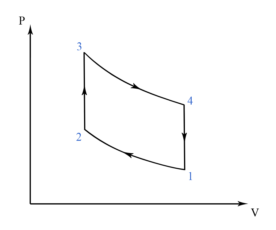
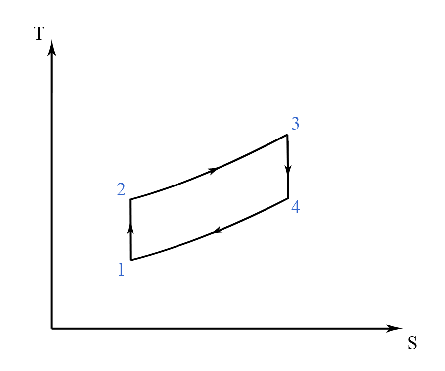
This cycle consists of an adiabatic compression of the WS (step $1-2$), followed by an isochoric heating, i.e. heating at constant volume (step $2-3$), then an adiabatic expansion of the WS (step $3-4$), and ended with an isochoric cooling which reverts the system back to its original condition (step $4-1$).

We know that the heat added or removed from the WS during a process at constant volume can be written as:

where $n$ is the number of moles of the WS, $C_V$ the heat capacity at constant volume, and $\Delta T$ the change in temperature. Hence, for the Otto cycle depicted in Figure 1 and Figure 2, we have that the heat supplied $Q_S$ is:

and the heat rejected $Q_R$ is:

Therefore, the thermal efficiency of the Otto cycle becomes (see equation 7):

from which we obtain:

As in this case the WS is treated as pure air, we can write for the adiabatic compression $1-2$ that:

and for the adiabatic expansion $3-4$ that:

In (13) and (14), $\gamma$ is the heat capacity ratio defined as:

where $C_P$ is the heat capacity at constant pressure, and $C_V$ the heat capacity at constant volume.

Equations (13) and (14) can also be written as:

and,

respectively. As $V_2=V_3$ and $V_4=V_1$ (steps $2-3$ and $4-1$ of the Otto cycle are isochoric - see Figure 1), we can rewrite equations (16) and (17) as:

and,

respectively, where $\displaystyle r=\frac{V_1}{V_2}=\frac{V_4}{V_3}$ is called the compression ratio.

By subtracting equation (18) from equation (19), we get that:

or furthermore, that:

which leads to:

By using (22) in equation (12), we obtain the thermal efficiency of the Otto cycle as:

It can be noted that the compression ratio $r$ for carburettor engines is about $7$, while for fuel injector engines it increases to around $10$. By using these figures, and also considering a value for the heat capacity ratio $\gamma$ of $1.25$, the thermal efficiency of a petrol/gasoline engine is found to be between $39\%$ and $44\%$. It can also be noted that for an Otto cycle engine, the ignition is usually performed by using a spark plug ("spark ignition").

Joule Cycle

The Joule cycle (also sometimes called the Brayton cycle, or the Constant Pressure cycle) is a thermodynamic cycle that describes the workings of the gas turbine engine. The Joule cycle is depicted on a $PV$ plot in Figure 3, and on a $TS$ plot in Figure 4.

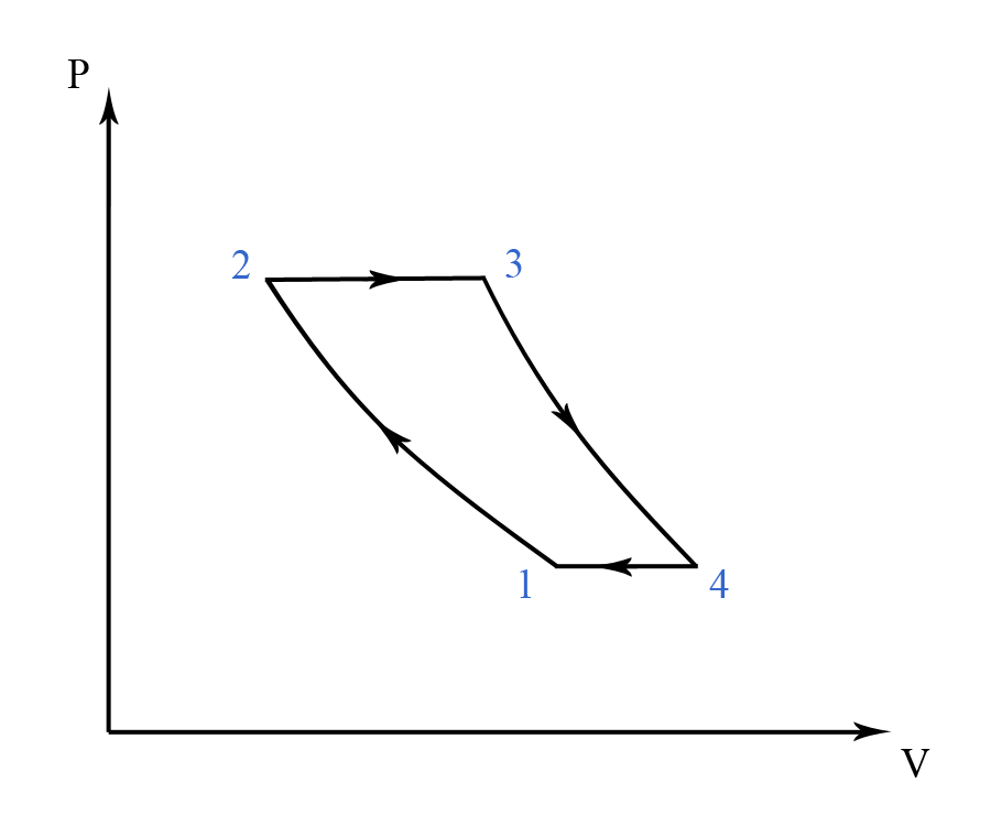
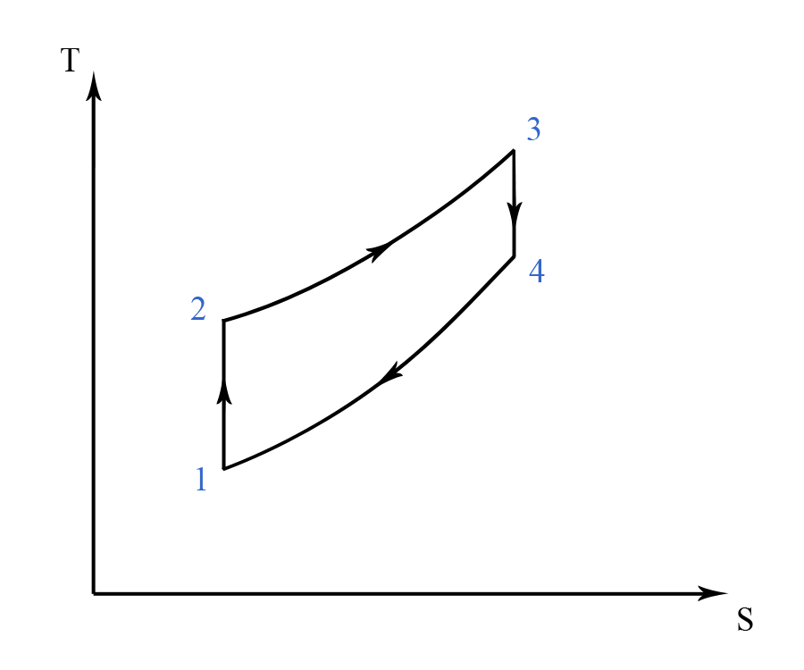
This cycle consists of a reversible adiabatic (i.e. isentropic) compression of the WS (step $1-2$), followed by an isobaric heating (i.e. heating at constant pressure) (step $2-3$), then a reversible adiabatic (isentropic) expansion of the WS (step $3-4$), and ended with an isobaric cooling which reverts the system back to its initial state (step $4-1$).

Similar to equation (8), we can write the heat added or removed from the WS during a process at constant pressure as:

where $n$ is the number of moles of the WS, $C_P$ the heat capacity at constant pressure, and $\Delta T$ the change in temperature. Therefore, for the Joule cycle depicted in Figure 3 and Figure 4, the heat supplied becomes:

and the heat rejected:

Hence, the thermal efficiency of the Joule cycle becomes (see equation 7):

from which we obtain:

As for the Joule cycle the WS is also treated as pure air, we can write for the isentropic compression $1-2$ that:

and for the isentropic expansion $3-4$ that:

where $\gamma$ is the heat capacity ratio (see equation 15).

Equations (29) and (30) can also be written as:

and,

respectively.

By raising equations (31) and (32) to the $\frac{\gamma - 1}{\gamma}$ power, we respectively get that:

and,

As $P_2=P_3$ and $P_4=P_1$ (steps $2-3$ and $4-1$ of the Joule cycle are isobaric - see Figure 3), we can rewrite equations (33) and (34) as:

and,

respectively, where $\displaystyle J=\frac{P_2}{P_1}=\frac{P_3}{P_4}$ is called the pressure ratio.

By subtracting equation (35) from equation (36), we get that:

or furthermore, that:

which leads to:

By using (39) in equation (28), we obtain the thermal efficiency of the Joule cycle as:

Diesel Cycle

The Diesel cycle is diagramed on a $PV$ plot in Figure 5, and on a $TS$ plot in Figure 6.

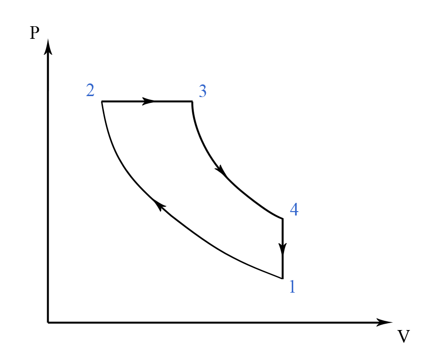
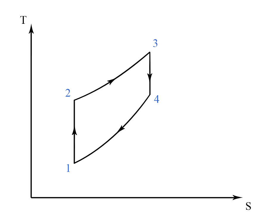
This cycle consists of a reversible adiabatic (isentropic) compression of the WS (step $1-2$), followed by an isobaric heating (step $2-3$), then a reversible adiabatic (isentropic) expansion of the WS (step $3-4$), and ended with an isochoric cooling which returns the system back to its original state (step $4-1$).

Taking into account equations (8) and (24), we can write the heat supplied (at constant pressure, step $2-3$) as:

and the heat rejected (at constant volume, step $4-1$) as:

where $n$ is the number of moles of the WS, $C_P$ the heat capacity at constant pressure, and $C_V$ the heat capacity at constant volume.

Therefore, the thermal efficiency of the Diesel cycle becomes (see equation 7):

which can also be written as:

where $\gamma$ is the heat capacity ratio (see equation 15).

As for the Diesel engine the WS is again treated as pure air, we can write for the isentropic compression $1-2$ that:

for the isobaric heating $2-3$ that:

and for the isentropic expansion $3-4$ that:

Equation (45) leads to:

which can also be written as:

where $\displaystyle r = \frac{V_1}{V_2}$ is the compression ratio.

From equation (46) we obtain:

which can also be written as:

where $\displaystyle \beta = \frac{V_3}{V_2}$ is the expansion ratio during heating (also called the cut-off ratio).

The temperature $T_3$ from (51) can further be expressed by considering the expression of $T_2$ from (49), as:

Equation (47) leads to:

which can also be written, by considering the expression of $T_3$ from (52), as:

We can write equation (54) in an analogous form as:

which leads to:

and furthermore, to:

Thus, we managed to express $T_2$, $T_3$, and $T_4$ all in function of $T_1$ (see equations 49, 52, and 57 respectively). By using these expression forms in equation (44), we get:

which leads to:

from which we obtain the thermal efficiency of the Diesel cycle as:

It can be noted that the ignition for the Diesel internal combustion engines is done by using a higher compression of the fuel, rather than by using a spark plug as in the case of gasoline powered Otto cycle engines. Therefore, the ignition for Diesel engines is sometimes called a "slow speed compression ignition", in contrast to the "spark ignition" of the Otto engines.

Example 1 [imperial]

Problem

An engine operates under a Diesel cycle with a top pressure of $642 \; psi$ ($lb/in^2$). The compression ratio is $18:1$, and the air at the start of compression is at $15 \; psi$ and $100^\circ F$. If $3 \; BTU$ are added during combustion and expansion in accordance to the law $PV^{1.25} = const.$, the clearance volume is $3 \; in^3$, the specific heat at constant pressure during combustion is $0.027 \; BTU/ft^3 ^\circ F$, and also if we are to ignore the fuel mass, find:

A) the pressure, volume, and temperature at each change point in the cycle;

B) the work output of the cycle (in $ft-lb$);

C) the thermal efficiency of the cycle.

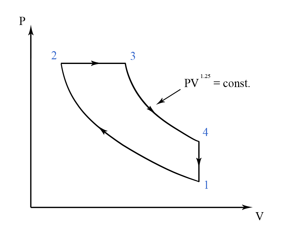
The corresponding Diesel cycle is diagramed on a $PV$ plot in Figure E1.

Workings

A) We are going to consider below each stage of the cycle separately.

Stage 1

We know from the hypothesis that the air at the start of compression is at $15 \; psi$ and $100^\circ F$. Therefore, the initial pressure is:

$$P_1 = 15 \; psi$$

(61)

while the initial temperature in kelvins ($K$) is:

$$T_1 = 100^\circ F = 310.77 \; K$$

(62)

We also know from the hypothesis that the compression ratio is $18:1$. As the compression ratio $r$ is defined as:

$$r = \frac{V_1}{V_2}$$

(63)

we obtain the initial volume:

$$V_1 = r V_2$$

(64)

which becomes, by taking into account that $r=18$ and that $V_2$ is the clearance volume ($V_2 = 3 \; in^3$):

$$V_1 = 54 \; in^3$$

(65)

Therefore $P_1 = 15 \; psi$, $V_1 = 54 \; in^3$, and $T_1 = 310.77 \; K$.

Stage 2

We have from the hypothesis that the top pressure is $642 \; psi$. Hence:

$$P_2 = 642 \; psi$$

(66)

Also from the hypothesis we have that the clearance volume is $3 \; in^3$. Thus:

$$V_2 = 3 \; in^3$$

(67)

By taking into account that:

$$\frac{P_1 V_1}{T_1} = \frac{P_2 V_2}{T_2}$$

(68)

we can write $T_2$ as:

$$T_2 = \frac{P_2 V_2}{P_1 V_1} T_1$$

(69)

By replacing the numerical values (see 61, 62, 65, 66, and 67), we obtain:

$$T_2 = \frac{642 \cdot 3}{15 \cdot 54} \cdot 310.77$$

(70)

from which:

$$T_2 = 736.52 \; K$$

(71)

Therefore $P_2 = 642 \; psi$, $V_2 = 3 \; in^3$, and $T_2 = 736.52 \; K$.

Stage 3

As step $2-3$ of the Diesel cycle is isobaric (see Figure E1), we have that:

$$P_3 = P_2$$

(72)

from which we obtain, by taking into account (66), that:

$$P_3 = 642 \; psi$$

(73)

For step $2-3$ of the cycle we can also write that:

$$Q_S = V_S C_P (T_3 - T_2)$$

(74)

where $Q_S$ is the heat supplied ($3 \; BTU$), $C_P$ the specific heat at constant pressure ($0.027 \; BTU/ft^3 ^\circ F$), and $(T_3 - T_2)$ is the temperature difference expressed in $^\circ F$, while $V_S$ is the quantity of gas which is present at a pressure of $P_S = 14.7 \; psi$ and at a temperature of $T_S = 60^\circ F$. In order to calculate $V_S$, we can write that:

$$\frac{P_S V_S}{T_S} = \frac{P_1 V_1}{T_1}$$

(75)

from which:

$$V_S = V_1 \frac{P_1}{P_S} \frac{T_S}{T_1}$$

(76)

Taking into account that:

$$T_S = 60^\circ F = 288.55 \; K$$

(77)

and also replacing the other numerical values (see 61, 62, and 65), we get that:

$$V_S = 54 \cdot \frac{15}{14.7} \cdot \frac{288.55}{310.77}$$

(78)

from which we obtain:

$$V_S = 51.11 \; in^3$$

(79)

By using the value of $V_S$ from (79) in equation (74), and also considering that $Q_S = 3 \; BTU$, $C_P = 0.027 \; BTU/ft^3 ^\circ F$, and that $1 \; ft^3 = 1728 \; in^3$, we get that:

$$3 = \frac{51.11}{1728} \cdot 0.027 \cdot (T_3 - T_2)$$

(80)

which leads to:

$$T_3 - T_2 = 3756.52^\circ F$$

(81)

or, by converting the temperature difference into kelvins, to:

$$T_3 - T_2 = 2342.17 \; K$$

(82)

As $T_2 = 736.52 \; K$ (see 71), we obtain $T_3$ as:

$$T_3 = 3078.69 \; K$$

(83)

Still for step $2-3$ of the cycle we can write that:

$$\frac{V_2}{T_2} = \frac{V_3}{T_3}$$

(84)

from which $V_3$ becomes:

$$V_3 = V_2 \frac{T_3}{T_2}$$

(85)

or, by replacing numerical values (see 67, 71, and 83):

$$V_3 = 3 \cdot \frac{3078.69}{736.52}$$

(86)

Equation (86) leads to:

$$V_3 = 12.54 \; in^3$$

(87)

Therefore $P_3 = 642 \; psi$, $V_3 = 12.54 \; in^3$, and $T_3 = 3078.69 \; K$.

Stage 4

As step $4-1$ of the Diesel cycle is isochoric (see Figure E1), we have that:

$$V_4 = V_1$$

(88)

from which we obtain, by taking into account (65), that:

$$V_4 = 54 \; in^3$$

(89)

As for step $3-4$ of the cycle we have that:

$$PV^{1.25} = const.$$

(90)

we can write:

$$P_3 V_3^{1.25} = P_4 V_4^{1.25}$$

(91)

from which $P_4$ becomes:

$$P_4 = P_3 \left( \frac{V_3}{V_4} \right)^{1.25}$$

(92)

or, by replacing numerical values (see 73, 87, and 89):

$$P_4 = 642 \cdot \left( \frac{12.54}{54} \right)^{1.25}$$

(93)

From equation (93) we obtain:

$$P_4 = 102.72 \; psi$$

(94)

We know that $\frac{PV}{T} = const.$ Therefore, we can divide equation (90) by $\frac{PV}{T}$ and still obtain a constant:

$$PV^{1.25} \div \frac{PV}{T} = const.$$

(95)

Equation (95) can also be written as:

$$PV^{1.25} \cdot \frac{T}{PV} = const.$$

(96)

from which we obtain, for step $3-4$ of the cycle, that:

$$TV^{0.25} = const.$$

(97)

Hence, we can write that:

$$T_3 V_3^{0.25} = T_4 V_4^{0.25}$$

(98)

from which $T_4$ becomes:

$$T_4 = T_3 \left( \frac{V_3}{V_4} \right)^{0.25}$$

(99)

or, by replacing numerical values (see 83, 87, and 89):

$$T_4 = 3078.69 \cdot \left( \frac{12.54}{54} \right)^{0.25}$$

(100)

From equation (100) we obtain:

$$T_4 = 2136.61 \; K$$

(101)

Therefore $P_4 = 102.71 \; psi$, $V_4 = 54 \; in^3$, and $T_4 = 2136.61 \; K$.

B) The work output $W$ of the cycle is given by:

$$W = (P_3 V_3 - P_2 V_2) + \left( \frac{P_3 V_3 - P_4 V_4}{n_1 - 1} \right) - \left( \frac{P_2 V_2 - P_1 V_1}{n_2 - 1} \right)$$

(102)

where $n_1 = 1.25$ (as $P_3 V_3^{1.25} = P_4 V_4^{1.25}$). In order to calculate $n_2$, we can write that:

$$P_1 V_1^{n_2} = P_2 V_2^{n_2}$$

(103)

which leads to:

$$\frac{P_2}{P_1} = \left( \frac{V_1}{V_2} \right)^{n_2}$$

(104)

By applying the $ln$ function to equation (104), we get:

$$ln \frac{P_2}{P_1} = n_2 ln \frac{V_1}{V_2}$$

(105)

from which we obtain:

$$n_2 = \frac{ln \frac{P_2}{P_1}}{ln \frac{V_1}{V_2}}$$

(106)

or, by replacing numerical values (see 61, 65, 66, and 67):

$$n_2 = \frac{ln \frac{642}{15}}{ln \frac{54}{3}}$$

(107)

Equation (107) leads to:

$$n_2 = 1.3$$

(108)

By replacing all the numerical values in equation (102) (see 61, 65, 66, 67, 73, 87, 89, and 94), and also taking into account that $n_1=1.25$, $n_2=1.3$ (see 108), and that $1 \; ft = 12 \; in$, we get the work done $W$ in $ft-lb$ as:

$$W = \left[ (642 \cdot 12.54 - 642 \cdot 3) + \left( \frac{642 \cdot 12.54 - 102.72 \cdot 54}{1.25 - 1} \right) - \left( \frac{642 \cdot 3 - 15 \cdot 54}{1.3 - 1} \right) \right] \cdot \frac{1}{12}$$

(109)

from which we obtain:

$$W = 1030.85 \; ft-lb$$

(110)

C) We know that the thermal efficiency is defined as:

$$\eta_{th} = \frac{W}{Q_S}$$

(111)

where $W$ is the work output, and $Q_S$ the heat supplied.

As, in our case, $W = 1030.85 \; ft-lb$ (see 110) and $Q_S = 3 \; BTU$, and also taking into account that $1 \; BTU = 778 \; ft-lb$, we get the thermal efficiency of the Diesel cycle as:

$$\eta_{th} = \frac{1030.85}{3\cdot 778}$$

(112)

from which we obtain:

$$\eta_{th} = 0.441$$

(113)

or, expressed as percentage:

$$\eta_{th} = 44.1\%$$

(114)

Solution

$P_1 = 15 \; psi$, $V_1 = 54 \; in^3$, $T_1 = 310.77 \; K$ $P_2 = 642 \; psi$, $V_2 = 3 \; in^3$, $T_2 = 736.52 \; K$ $P_3 = 642 \; psi$, $V_3 = 12.54 \; in^3$, $T_3 = 3078.69 \; K$ $P_4 = 102.71 \; psi$, $V_4 = 54 \; in^3$, $T_4 = 2136.61 \; K$ $W = 1030.85 \; ft-lb$ $\eta_{th} = 44.1\%$