CodeCogs

An analysis of surge tanks (Frictionless and flow with allowance made for friction)

You're viewing an older version of this page (#3360). View the current version.

Surge Tanks

The Surge tank or stand pipe is used in turbine installations to reduce the pressure surges which occur when the load on the turbine is suddenly changed. It must be sited as close to the turbine as possible to avoid surges in the length of pipe between the surge tank and the turbine.

When the flow to the turbine is reduced, water flows into the surge tank and conversely for increased load , the initial extra water required is from the surge tank. The tank should not overflow when the turbine is suddenly shut down, nor allow air to be drawn into the system following a sudden increase in demand.

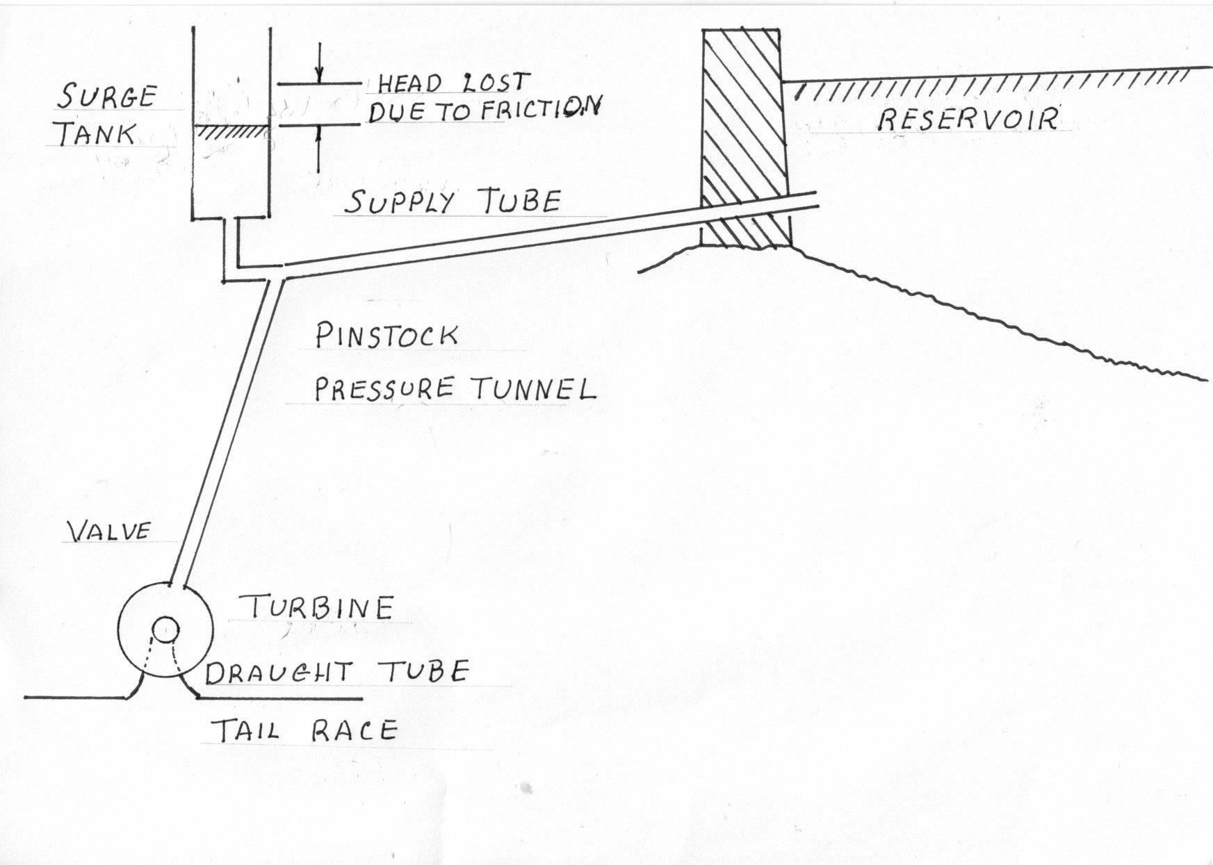
Instantaneous Closure neglecting friction

Blank

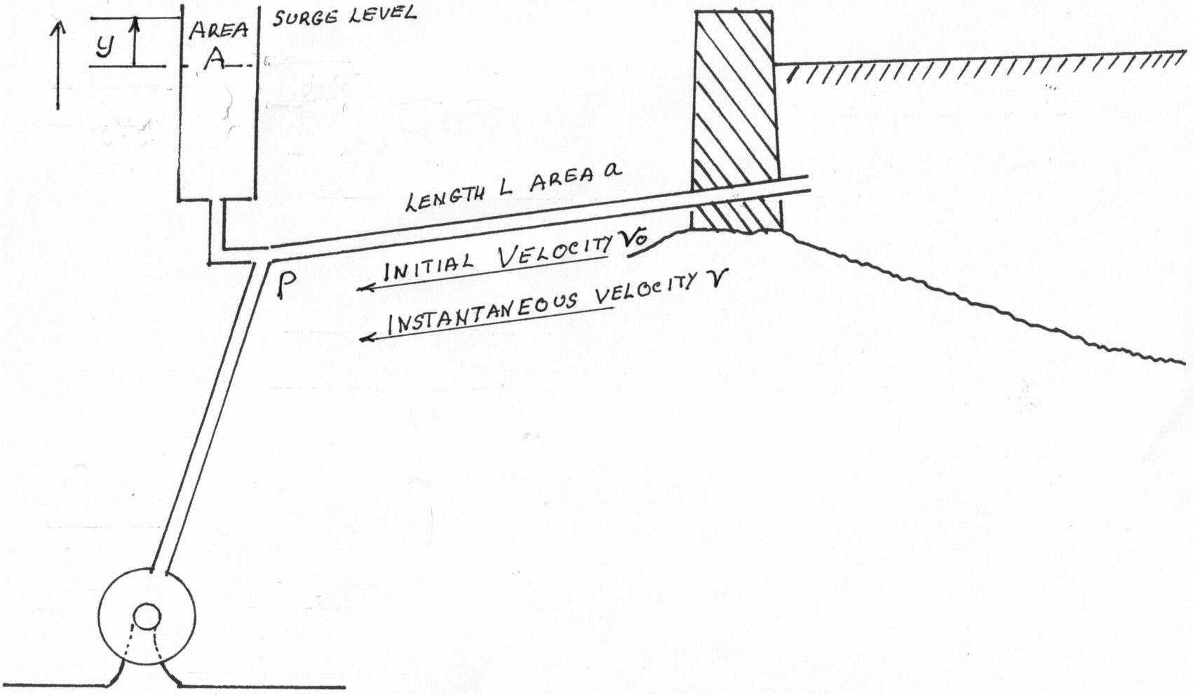
Let

$R = \frac{Surge\;tank\;area\;"A"}{Pipe\;line\;area\;"a"}$
v = the instantaneous velocity in the pile line t secs. after the change in load
y = The height of the surge level above the surface of the reservoir t secs. after the change in load.
w = density of water

At time t the pressure at P above normal flow conditions = w y

By Newtons second Law
The pressure force on the water column in the pipe line = Mass * Acceleration

$w\,y\,a=\frac{w\,a\,L}{g}\times - \frac{dv}{dt}$

(1)

$\therefore\;\;\;\;y = -\frac{L}{g}\;\frac{dv}{dt}$

(2)

(y is called the Acceleration or Inertia head )

By Mass Continuity
Flow in the surge tank = Flow in the pipe, i.e.

$A \frac{dy}{dt} = a\,v$

(3)

$v = \frac{A}{a}\,\frac{dy}{dt} = R\;\frac{dy}{dt}$

(4)

Differentiate

$\frac{dv}{dt} = R\,\frac{d^2y}{dt^2}$

(5)

Substituting in equation (3)

$y = - \frac{L}{g}\times R\,\frac{d^2y}{dt^2}$

(6)

$\therefore\;\;\;\;\;\frac{d^2y}{dt^2} + \frac{g}{L\,R}y=0$

(7)

But this is the equation for simple harmonic motion whose solution is:-

$y = C cos\sqrt{\frac{g}{L\,R}t^2} + D sin\sqrt{\frac{g}{L\,R}}t$

(8)

When t = 0 y = 0 and by inspection C = 0

$Hence\;\;\;\;\;y=D \sqrt{\frac{g}{L\,R}.}\times \;t$

(9)

Differentiate equation (10)

$\frac{dy}{dt} = D\sqrt{\frac{g}{L\,R}}\;cos\sqrt{\frac{g}{L\,R}}\times t$

(10)

But from equation (6) when t=0

$\frac{dy}{dt} = \frac{v_0}{R}$

(11)

and also

$\cos \sqrt{\frac{g}{L\,R}}=1$

(12)

$\therefore\;\;\;\;\frac{v_0}{R} = D\sqrt{\frac{g}{L\,R}}$

(13)

$\therefore\;\;\;\;D = v_0\;\;\sqrt{\frac{L}{g\,R}}$

(14)

Substitute in equation (10)

$y = v_0 \sqrt{\frac{L}{g\,R}} cos \sqrt{\frac{g}{L\,R}}$

(15)

If T is the period of a complete oscillation,

$when\;\;\;t=\frac{T}{2}\;\;\;\;\;\;\;\;y=0$

(16)

$\therefore\;from\;equation\;(\;) \;\;\;since\;\;\;\;D\neq 0$

(17)

$sin\;\sqrt{\frac{g}{L\,R}}\times \frac{T}{2}=0$

(18)

$\therefore\;\;\;\;\;\sqrt{\frac{g}{L\,R}}\times \frac{T}{2}=\pi$

(19)

$\therefore\;\;\;\;\;T=2\pi \sqrt{\frac{L\,R}{g}}$

(20)

From equation (6)

$v=R \frac{dy}{dt}=R v_0 sqrt{\frac{L}{gR}}\times \sqrt{\frac{g}{LR}} cos\sqrt{\frac{g}{LR}}\times t$

(21)

$\therefore\;\;\;\;\;v = v_0\;cos\sqrt{\frac{g}{LR}}\times t$

(22)

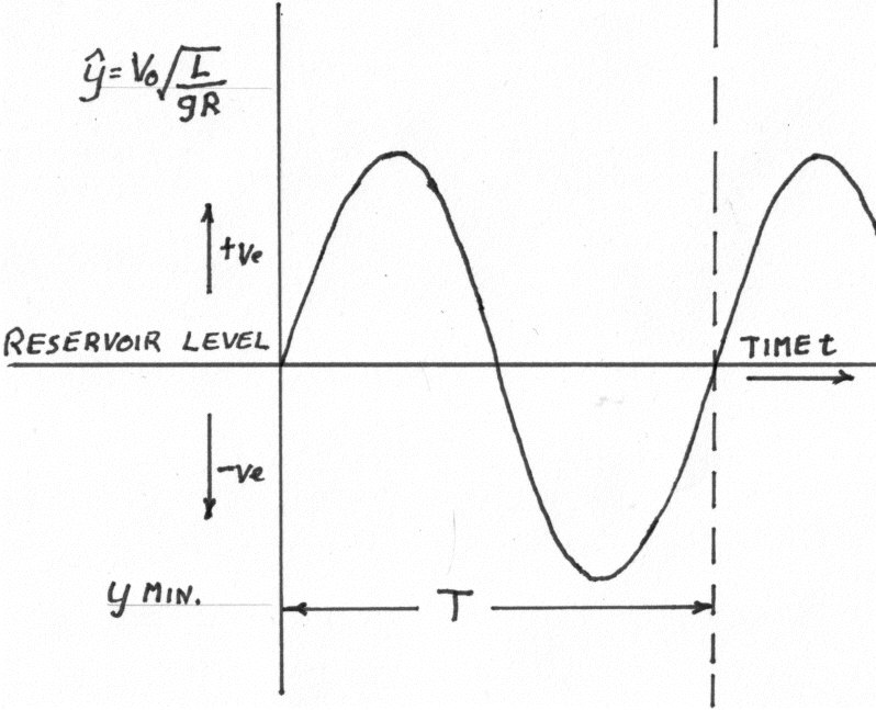
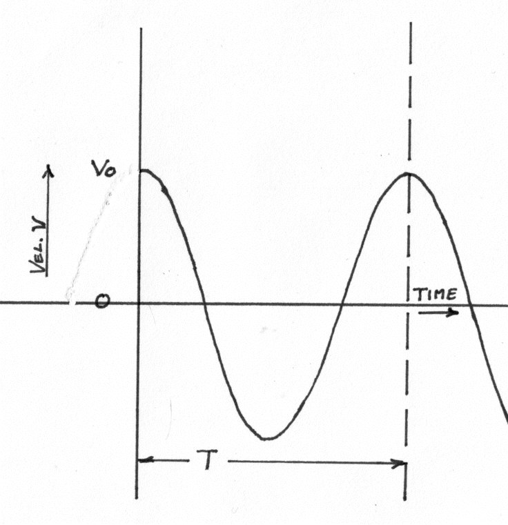
The following two graphs show the variation of both y and v with time.

NOTES

The maximum surge height occurs at time t, i.e. $\left(\frac{T}{4} \right)=\frac{\pi }{2}\sqrt{\frac{LR}{g}}$

$\hat{y}=v_0 \sqrt{\frac{L}{gR}}$

(23)

A large value of R i.e. a large surge tank area means a small $\hat{y}$ but the longer the period T.
Changes in reservoir level and the inertia of the water column in the surge tank have been neglected.

A Sudden Complete Valve Closure allowing for Friction.

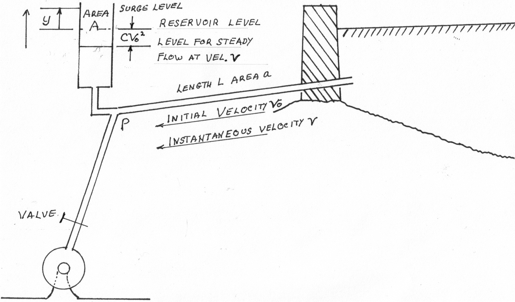
At the initial steady flow state the level in the surge tank will be below the reservoir level by an amount equal to the friction head lost in the pipe.

$=\frac{4flv_0^2}{2dg}\;\;\;where\;n\approx 2$

(24)

This is usually written as $C v_0^2$ where C is a constant for the pipe line.

At a time t secs, after closure the surge level is at a hight y above the reservoir level and the pipe velocity is v.

For steady flow at velocity v the level in the surge tank would be $C v^2$ below the reservoir level.

Thus the excess pressure head at P causing the deceleration of the water column is $(y+C\,v^2)$

Therefore by Newton's second Law: "Pressure force = mass X acceleration"

$w(y + C\,v^2)\;a=\frac{w\,a\,l}{g}\;\times - \frac{dv}{dt}$

(25)

$\therefore\;\;\;\;\;y + C\,v^2=- \frac{l}{g}\;\;\frac{dv}{dt}$

(26)

But by continuity

$a\,v=A\;\frac{dy}{dt}\;\;\;or\;\;\;v=R\;\frac{dy}{dt}$

(27)

Hence

$\frac{dv}{dt}=R\;\frac{d^2v}{dt^2}$

(28)

Substituting from equations (27) and(28) in (26)

$\therefore\;\;\;\; y+C\left(R\,\frac{dy}{dt} \right)^2=- \frac{L}{g}\;R\;\frac{d^2y}{dt^2}$

(29)

i.e.

$\frac{d^2y}{dt^2}+\frac{CRg}{L}\;\left(\frac{dy}{dt} \right)^2+\frac{g}{LR}=0$

(30)

This is insoluable as it stands since we can not deal with the friction term.

To eliminate t

$\frac{dv}{dt}=\frac{dv}{dy} \frac{dy}{dt} = \frac{v}{R} \frac{dv}{dy}$

(31)

But

$v\,\frac{dv}{dy} = \frac{1}{2} \frac{d(v^2)}{dy}$

(32)

therefore

$\frac{dv}{dt} = \frac{1}{2R}\times \frac{d(v^2)}{dy}$

(33)

Substitute in equation (26)

$y+Cv^2=-\frac{L}{2gR}\times \frac{d(v^2)}{dy}$

(34)

$\frac{d(v^2)}{dy} + \frac{2gRC}{L}\times v^2 + \frac{2gR}{L}y=0$

(35)

The solution of this equation is:-

$v^2=K\;e^\frac{-\,2gRCy}{L} - \frac{y}{C} + \frac{L}{2gRC^2}$

(36)

The evaluation of the constant K when t = 0 $v=v_0$ and $y=-Cv_0^2$

$\therefore\;\;\;\;\;K = -\frac{L}{2gRC^2} e^\frac{- 2gRC^2\,v_0^2}{L}$

(37)

$\therefore\;\;\;\;\;v^2 = -\frac{L}{2gRC^2} e^{\frac{- 2gRC}{L}(y\,+\,CV_0^2)}$

(38)

The hight of the first maximum surge can then be found by putting v = 0 and y = y(max.) in the above equation. The equation can then only be solved by trial and error but a first approximation neglecting friction and using $\hat{y}=v_0\sqrt{\frac{L}{gR}}$ will save work!

First Minimum Surge.

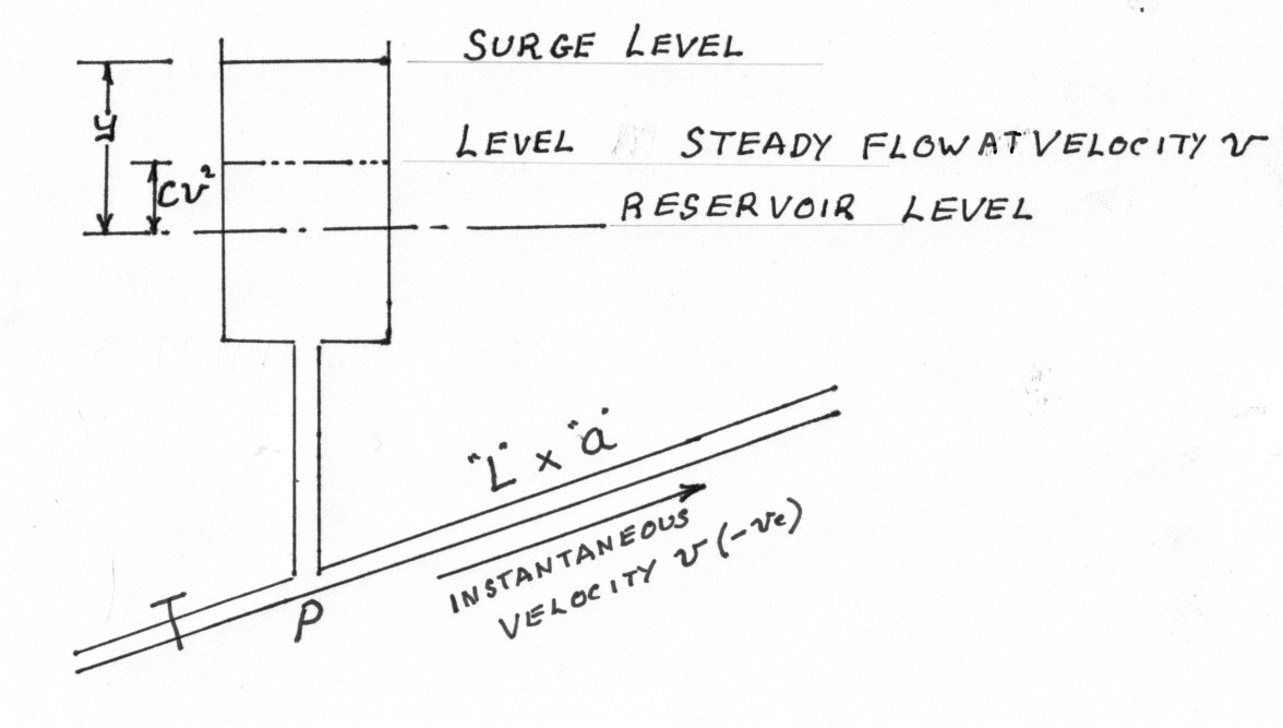
Head at p accelerating the column towards the reservoir is $y - Cv^2$ .

Equation (26) now becomes:-

$y-Cv^2 = -\frac{L}{g} \frac{dv}{dt}$

(39)

and by continuity:-

$-av = A\times - \frac{dv}{dt}$

(40)

$v = R\;\frac{dy}{dt}$

(41)

NOTE: the net effect of the flow reversal on the above equations is to change the sign of the $C\;v^2$ term, so the equations generated, during the consideration for sudden complete closure are modified as follows.

$\frac{d^2y}{dt^2} - \frac{CRg}{L}\left(\frac{dy}{dt} \right)^2 + \frac{g}{LR}y = 0$

(42)

$\frac{d(v^2)}{dy} - \frac{2gRC}{L}v^2 + \frac{2gR}{L}y=0$

(43)

Putting v = 0 when y = y max gives K

$v^2-\left(\frac{\hat{y}}{C}+\frac{L}{2gRC^2}\right ) e^{\frac{2gRC}{L}(\hat{y}\,-\,y)} + \frac{y}{C} + \frac{L}{2gRC^2}$

(44)

The following graphs show the variations of y and v with time.

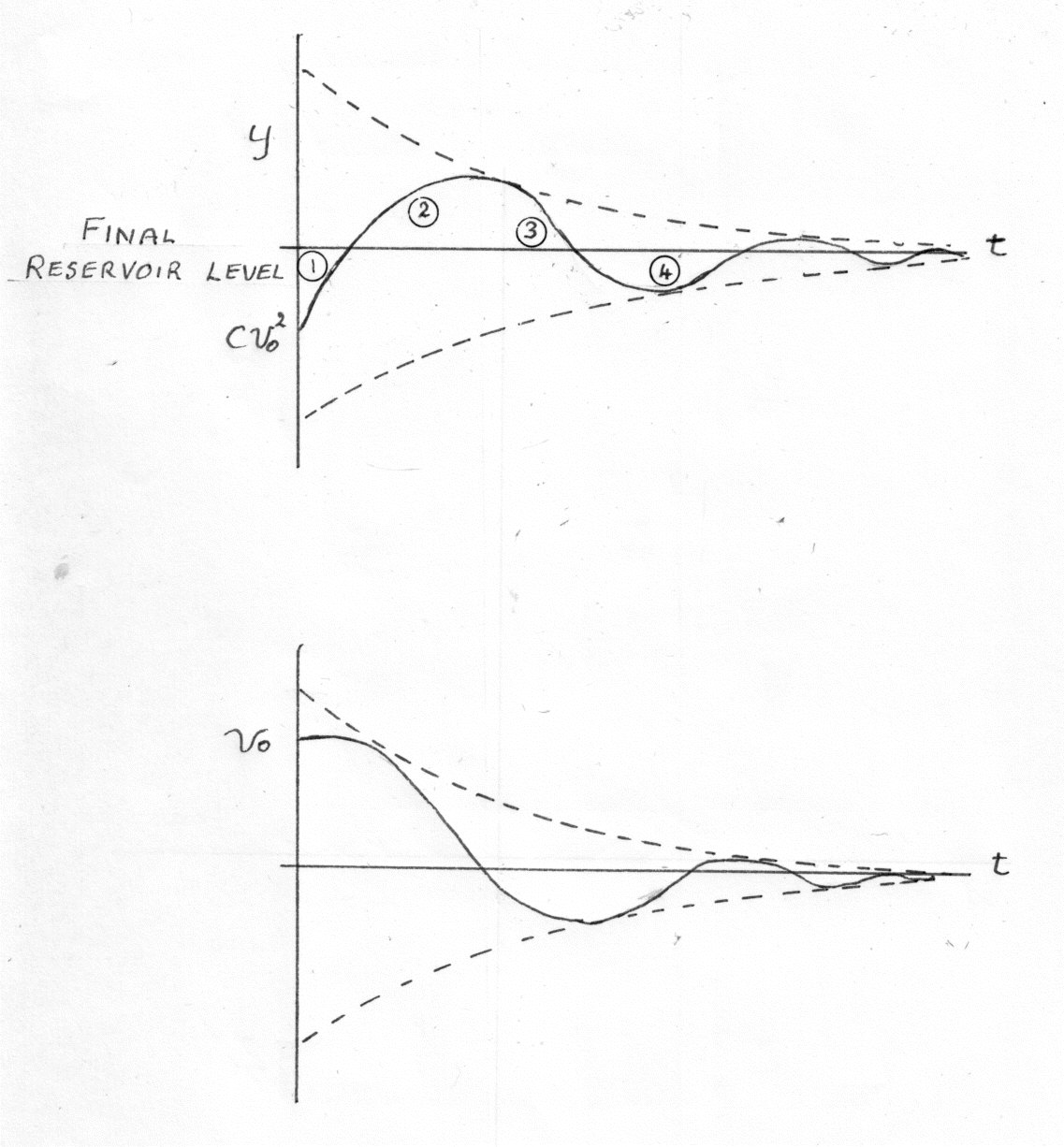
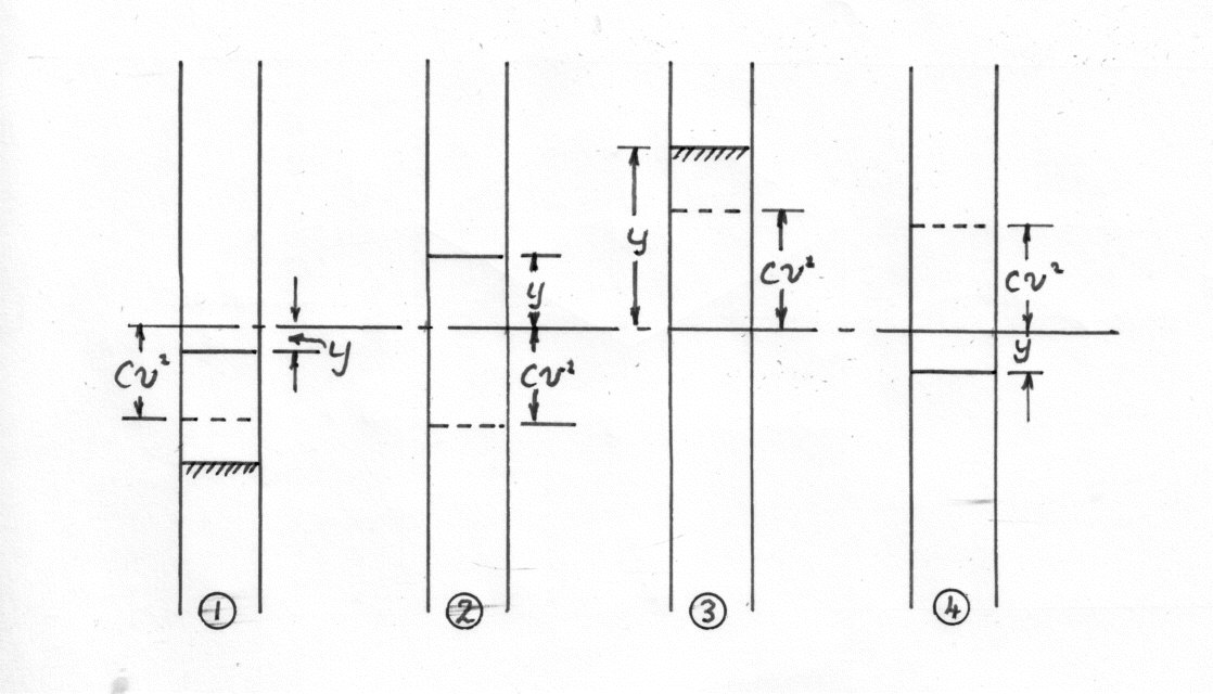
In all the above theory y is measured positively upwards from the reservoir level. $\frac{dy}{dt}$ is positive or negative depending upon whether the surge level is rising or falling. v is positive or negative depending whether the flow is towards the surge tank or away from it. $Cv^2$ is added when the flow is towards the surge tanks and is subtracted if the flow is towards the reservoir.

Gradual Valve Closure

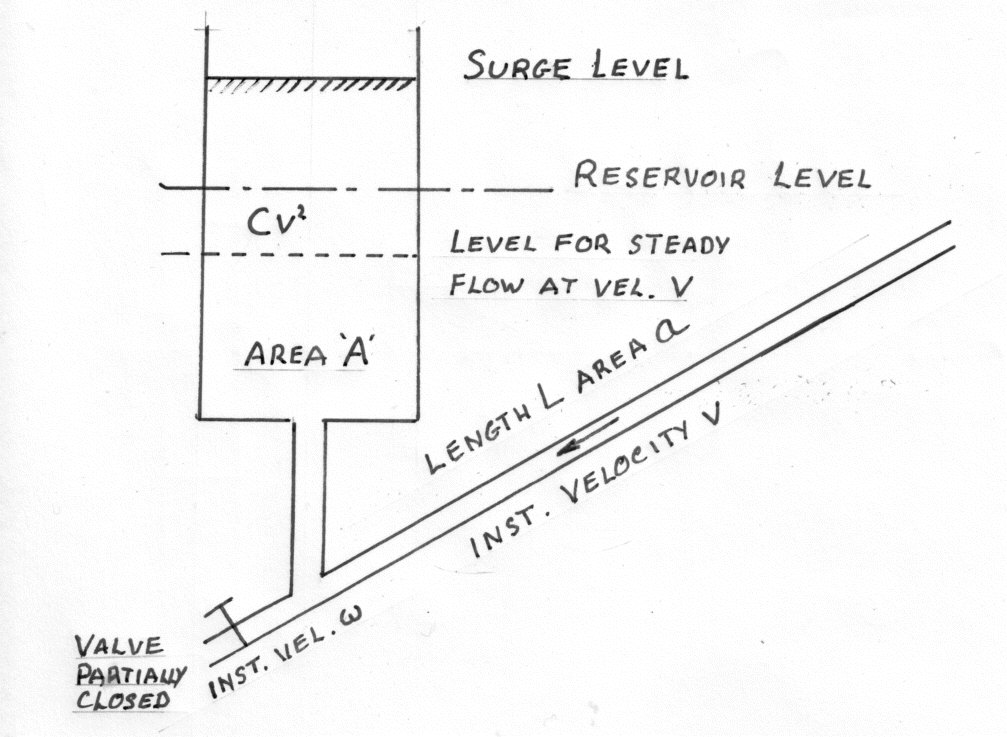
Consider the instantaneous conditions at a time t as shown. The head at P decelerating the column is

$y + Cv^2$

(45)

and

$y+Cv^2 = - \frac{L}{g} \frac{dv}{dt}$

(46)

By Continuity

$a(v-\omega ) = A \frac{dy}{dt}$

(47)

$v-\omega = R \frac{dy}{dt}$

(48)

After the valve has closed in a time t\_c, ω remains zero and the equation becomes

$v = R \frac{dy}{dt}\;\;\;\;\;\;as\;before$

(49)

This can only be dealt with by numerical integration and even then the variation of ω with time must be known. It is usual to assume that ω decreases uniformly from v\_0 to zero in a time t\_c. i.e. at a time t

$\omega = v_0 \left(1-\frac{t}{t_c} \right)$

(50)

Sudden or Gradual Partial Closure.

Equations (3) and (6) still apply but ω does not now fall to zero.

For a sudden partial closure ω is assumed to fall instantaneously to the new steady value. For a gradual partial closure ω is assumed to fall linearly with time to the new constant value ω\_c at time t.

i.e.

$\omega =\omega _c + (v_0 - \omega _c)\left(1 - \frac{t}{t_c} \right)$

(51)

Sudden Valve Opening on Increased Load.

NOTE: Assume tat the velocity at the valve increases instantaneously to the final steady velocity ω\_c

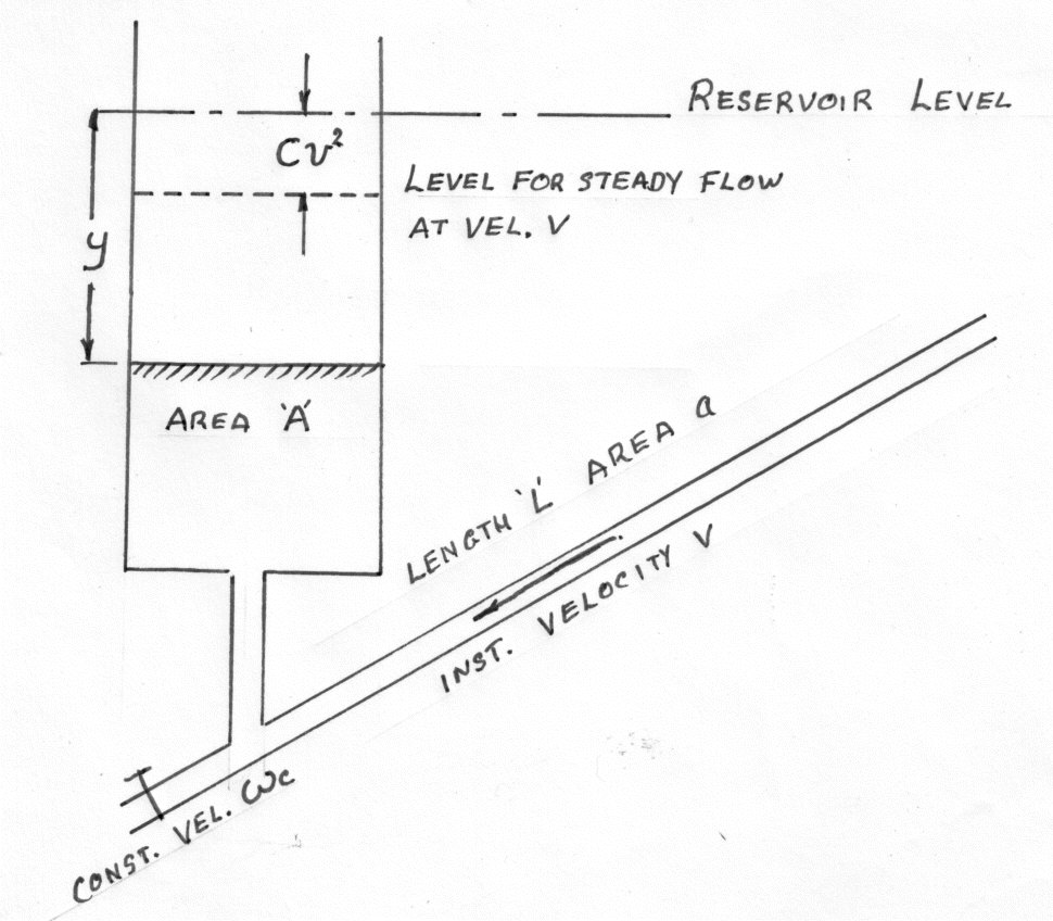
Consider the position shown. Take y as positive downwards.

$\left(y-Cv^2 \right)=\frac{L}{g} \frac{dv}{dt}$

(52)

$a\left(\omega _c - v \right)=A \frac{dy}{dt}$

(53)

$\left(\omega _c - v \right) = R \frac{dy}{dt}$

(54)

Variations of y and v with time

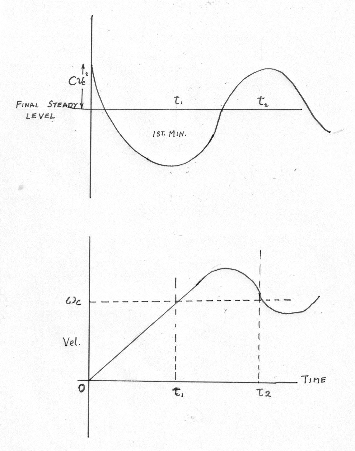
NOTES

The interaction of the turbine governing mechanism and the surge tank frequency must be studied so that surges are damped out by friction and not perpetuated and amplified by the action of the governor. The following equation gives the critical area ratio for stability.

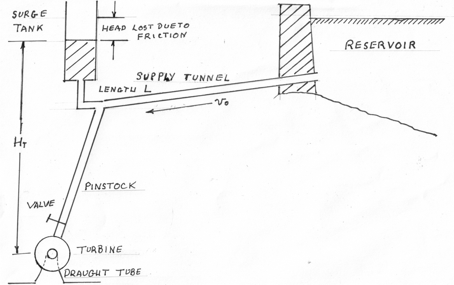
$R_{critical} = \frac{L}{H_tCv_0^2}\times \frac{v_0^2}{2g}$

(55)

H\_t is the initial steady flow level in the surge tank above the turbine gate.