Univariate

A function expresses the idea that one quantity (the argument of the function) completely determines another quantity (the value).

Interpolation is a method of constructing new data points within the range of a discrete set of known data points.

A polynomial is an expression of finite length constructed from variables and constants, using only the operations of addition, subtraction, multiplication, and non-negative integer exponents.

Carl Runge (1856-1927) was a German mathematician, physicist, and spectroscopist. He was co-developer and co-eponym of the Runge-Kutta method, in the field of what is today known as numerical analysis.

Univeriate curve-fitting, interpolation, polynomial, spline, Akima

View versions (2)

Univariate interpolation is an area of curve-fitting which, as opposed to univariate regression analysis, finds the curve that provides an exact fit to a series of two-dimensional data points.It is called univariate as the data points are supposed to be sampled from a one-variable function. Compare this to multivariate interpolation, which aims at fitting data points sampled from a function of several variables.

Formally speaking, consider a series of $N$ data points $(x_1, y_1), (x_2, y_2), \ldots, (x_N, y_N)$ and, for the sake of simplicity, consider that $x_1 < x_2 < \ldots < x_N$ , i.e. the points are distinct and are in increasing order with respect to $x$ . By interpolating these data points we mean finding a function $f : [x_1, x_n] \to \mathbb{R}$ such that:

$f(x_1) = y_1, \quad f(x_2) = y_2, \quad \ldots \quad f(x_N) = y_N.$

(1)

To make things even clearer, consider the following example. Let the data points be $(0, 0), (\pi, 0), (2 \pi, 0)$ , shown in red in the image below.

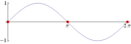
As you may notice, we can choose $f(x) = \sin(x)$ to be the interpolation function, which is also shown in blue in the previous graph. It clearly satisfies the constraints of equation (1), but it's not necessarily the most straightforward choice. We might as well choose the constant function $f(x) = 0$ , which also satisfies the constraints of equation (1) and is therefore a valid interpolation function for the given data points.

As a conclusion, we are allowed to choose any type of function as long as it provides an exact fit to the given data points. Our choice should be based on some prior knowledge of the phenomena which generated that series of points.

Polynomial interpolation

In the following, let us assume that the interpolation function is polynomial, i.e. $f$ is of the type

$f(x) = a_0 + a_1 x + a_2 x^2 + \ldots + a_k x^k,$

where $k$ is called the degree of $f$ and $a_0, a_1, \ldots, a_k$ are some real numbers, called the coefficients of $f$ . In order to find the expression for $f$ , it suffices to find its coefficients. We are able to find them by writing the constraints of equation (1) in our particular case:

$\left\{\begin{array}{ccccccccccccc} f(x_1) &=& y_1 &= &a_0 &+ &a_1 x_1 &+ &a_2 x_1^2 &+ &\ldots &+ &a_k x_1^k \\ f(x_2) &=& y_2 &= &a_0 &+ &a_1 x_2 &+ &a_2 x_2^2 &+ &\ldots &+ &a_k x_2^k \\ \ldots && \ldots && \ldots \\ f(x_N) &=& y_N &= &a_0 &+ &a_1 x_N &+ &a_2 x_N^2 &+ &\ldots &+ &a_k x_N^k \\ \end{array}\right.$

This is a system of linear equations with $k + 1$ unknowns, $a_0, a_1, \ldots, a_k$ and $N$ equations. In order to have a unique solution, we need to require that $k + 1 = N$ , or $k = N - 1$ ; that is, we require that the degree of $f$ should be equal to the number of data points minus one. However, this is a worst case scenario since, by solving the above linear system, one may obtain $a_k = 0$ which will decrease the degree of $f$ by one, and so on. As a general rule, the degree of $f$ will be strictly less than the number of given data points.

The function $f$ determined by solving the above system of linear equations is called the interpolation polynomial for the series of data points $(x_1, y_1), (x_2, y_2), \ldots, (x_N, y_N)$ .

Directly solving this system of linear equations comes down to finding the inverse of its corresponding matrix, which might become computationally expensive. Another easier way of finding the coefficients of $f$ is by writing it in the Lagrange form :

$f(x) = y_1 L_1(x) + y_2 L_2(x) + \ldots + y_N L_N(x),$

where $L_i$ is defined through

$L_i(x) = \mathop{\prod_{j = 1}^n}_{j \neq i} \left(\frac{x - x_j}{x_i - x_j}\right),$

for all $i = 1, 2, \ldots, N$ . It can easily be shown that $L_i(x_i) = 1$ and $L_i(x_j) = 0$ , for all $j \neq i$ ; therefore $f(x_i) = y_i$ , so $f$ satisfies the constraints of equation (1). This provides a method of computing the interpolation polynomial $f$ known as Lagrange interpolation, which is also implemented as the component Lagrange.

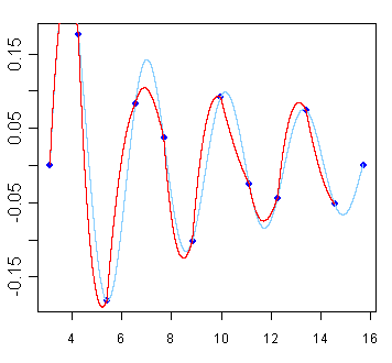
Consider the function

$\psi(x) = \frac{\sin(2x)}{x}$

with $x$ in the interval $[\pi, 4 \pi]$ and let us sample 12 equidistant points from this function. Applying Lagrange interpolation on this series of data points results in the following approximation (shown in red):

{Runge's phenomenon}

When trying to estimate the error between the original function, from which the series of data points has been sampled, and the polynomial interpolation function $f$ , one may notice the following phenomenon. Conside the Runge function:

$R(x) = \frac{1}{1 + 25 x^2}$

Now, consider a series of $N$ equidistant points $(x_1, y_1), (x_2, y_2), \ldots, (x_N, y_N)$ between $-1$ and $1$ , where

$x_i = -1 + (i - 1)\frac{2}{N - 1},\quad y_i = f(x_i),$

for all $i = 1, 2, \ldots, N$ .

Runge proved that the polynomial interpolation function corresponding to this set of data oscillates toward the end points of the interval $[-1, 1]$ . More than that, the interpolation error at the ends of the interval tends to increase to infinity as you increase the number of equidistant data points. This is also known as Runge's phenomenon.

In the image below, the Runge function is depicted in red, while the 5-th degree (6 points) and 9-th degree (10 points) interpolation polynomials are shown in blue and green, correspondingly. Notice how the approximation error at the ends of the interpolation interval increases with the degree of $f$ , or with the number of given equidistant points.

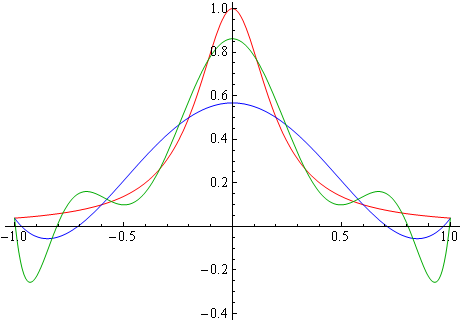
As a conclusion, polynomial interpolation in the case of a large number of equidistant points might generate large approximation errors toward the end points of the interpolation interval. This phenomenon can be avoided using spline interpolation, which is the subject of the next section.

Spline interpolation

Spline interpolation is somehow a generalization of polynomial interpolation, in that we do not necessarily have to find a single polynomial function to fit the data over the entire interval, but we rather try to find several polynomial functions to fit the data over each subinterval determined by two consecutive data points, while obeying some smoothness conditions.

One of the advantages of this generalization is that the resulting interpolation function is less wiggly, as in the case of e.g. Lagrange interpolation.

Formally, consider the series of $N$ data points in the above paragraphs, which are distinct and ordered increasingly with respect to $x$ . A spline interpolation function of degree $d \geq 1$ for the given data points is a function $S : [x_1, x_N] \to \mathbb{R}$ which satisfies the following conditions

$S(x) = p_i(x)$ , for all $x \in [x_i, x_{i+1}]$ and all $i = 1, 2, \ldots, N - 1$ , where $p_i$ is some polynomial function with degree less than or equal to $d$
the derivatives of $S$ up to the order $n-1$ are all continuous in the given data points, which basically means that for all $i = 1, 2, \ldots, N - 1$ we require that:

$\left\{ \begin{array}{lcl} p_i(x_{i+1}) &=& p_{i+1}(x_{i+1}) \\ p_i'(x_{i+1}) &=& p_{i+1}'(x_{i+1}) \\ p_i''(x_{i+1}) &=& p_{i+1}''(x_{i+1}) \\ \ldots&& \ldots \\ p_i^{(n-1)}(x_{i+1}) &=& p_{i+1}^{(n-1)}(x_{i+1}). \end{array} \right.$

Without getting into further technical details, we mention that the above relations lead to an under-determined system of linear equations. In order to obtain solution uniqueness to this system and completely determine the spline interpolation function $S$ , $n - 1$ more relations need to be set.

In the case of cubic splines ( $n = 3$ ), notice that we need $n - 1 = 2$ additional relations to determine $S$ . These are given, for example, by $p_1''(x_1) = p_2''(x_3) = 0$ . In this case, $S$ is called a natural cubic spline. Other kinds of cubic splines can be obtained using other pairs of conditions.

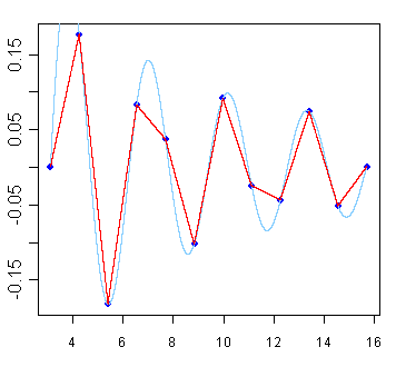
In the case when $n = 1$ , $S$ is piecewise linear and the method is called linear interpolation, which is also implemented as Linear. In the graph below you can see the way linear interpolation (in red) works in the case of 12 equidistant points sampled from the function $\psi$ , previously defined.

In the case when $n = 3$ , $S$ is comprised of cubic polynomial functions on each subinterval and the method is called cubic interpolation, which is also implemented as Cubic. The following graph shows the cubic spline (in red) for the $\psi$ function.

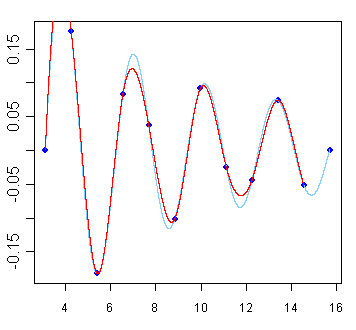
Notice that higher degree spline interpolation results in smaller approximation errors. However, in order to escape from Runge's phenomenon, instead of increasing the degree of the spline, it is prefered to increase the number of data points. This can be achieved, for instance, by doing further experiments and obtaining further input data.

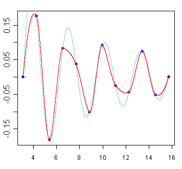
Akima interpolation is a particular type of third-degree spline interpolation, also implemented as Akima. Its main advantage is that, as opposed to cubic spline interpolation, it is applicable on successive intervals, so it does not require solving large systems of linear equations. Apart from being more computationally efficient, it also provides a more natural interpolation curve, closer to human intuition.

The graph below shows the Akima interpolation curve for the $\psi$ function.

Author

author}

Blank

author}

Lucian Bentea (August 2008)

References

George M. Philips, Interpolation and Approximation by Polynomials, Springer-Verlag, New York, 2003.
http://en.wikipedia.org/wiki/Curve_fitting
http://en.wikipedia.org/wiki/Interpolation
http://en.wikipedia.org/wiki/Runge%27s_phenomenon
http://en.wikipedia.org/wiki/Spline_interpolation
Hiroshi Akima, A New Method of Interpolation and Smooth Curve Fitting Based on Local Procedures, Journal of the ACM, Vol. 17, No. 4, October 1970, pp. 589-602.
http://www.iue.tuwien.ac.at/phd/rottinger/node60.html