CodeCogs

An introduction to Shear Force and Bending Moments in Beams

You're viewing an older version of this page (#3552). View the current version.

Shearing Force

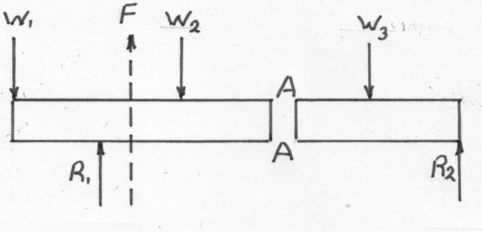
The shearing force (SF) at any section of a beam represents the tendency for the portion of the beam on one side of the section to slide or shear laterally relative to the other portion.

The diagram shows a beam carrying loads $W_1$ , $W_2$ and $W_3$ . It is simply supported at two points with reactions $R_1$ and $R_2$ .

Assume that the beam is divided into two parts by a section XX the loads and reaction acting on the left of AA is F vertically upwards.

Since the whole beam is in equilibrium, the resultant force to the right of AA must be F downwards. F is called the Shearing Force at the section AA, and is defined defined as:

The shearing force at any section of a beam is the algebraic sum of the lateral components of the forces acting on either side of the section.

Where forces are neither in the lateral or axial direction they must be resolved in the usual way and only the lateral components use to calculate the shear force.

Bending Moments

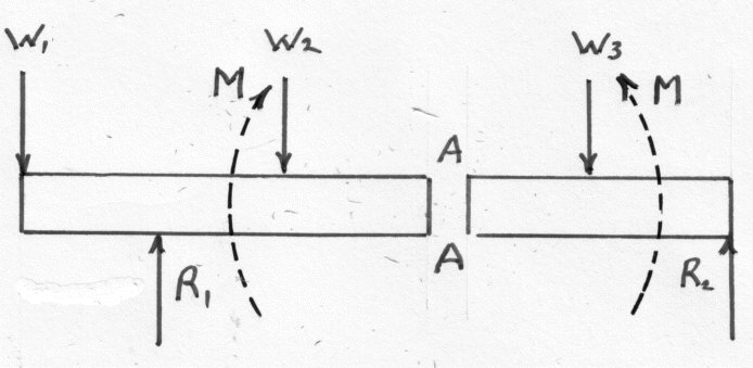
If the Bending moments (BM) of the forces to the left of AA are clockwise then the bending moment of the forces to the right of AA must be anticlockwise.

Bending Moment at AA is defined as the algebraic sum of the moments about the section of all forces acting on either side of the section.

Bending moments are considered positive when the moment on the left portion is clockwise and on the right anticlockwise.

A positive bending moment is also referred to as a sagging bending moment as it tends to make the beam concave upwards at AA. A negative bending moment is termed hogging.

Types of Load

A beam is normally horizontal and the loads vertical. Other cases which occur are considered to be exceptions.

A Concentrated load is one which can be considered to act at a point although of course in practice it must be distributed over a small area.

A Distributed load is one which is spread in some manner over the length or a significant length of the beam. It is usually quoted at a weight per unit length of beam. It may either be uniform or vary from point to point.

Types of Support

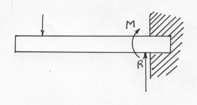
A Simple or free support is one upon which the beam is rested and that exerts a reaction on the beam. It is normal to assume that the reaction acts at a point although it may in fact act act over a short length of beam.

A Built-in or encastre' support is frequently met. The effect is to fix the direction of the beam at the support. In order to do this the support must exert a "fixing" moment M and a reaction R on the beam. A beam which is fixed at one end in this way is called a Cantilever. If both ends are fixed in this way the reactions are not statically determinate.

In practice it is not usually possible to obtain perfect fixing and the fixing moment applied will be related to the angular movement of the support. When in doubt about the rigidity it is safer to assume that the beam is freely supported.

The Relationship between w, F, and M

In the following diagram $\delta x$ is the length of a small slice of a loaded beam at a distance x from the origin O

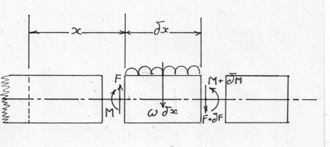
Let the shearing force at the section $x$ be $F$ and at $x=\delta x$ be $F+\delta F$ . Similarly the bending moment is $M$ at $x$ and $M+\delta M$ at $x+\delta x$ . If w if the mean loading along the length $\delta x$ , then the total load is $w \delta x$ , acting approximately (exactly if uniformly distributed) through the centre C. The element must be in equilibrium under the action of these forces and couples and the following equations can be obtained:-

Taking Moments about C

$M+F \frac{\delta x}{2} + (F + \delta F) \frac{\delta x}{2} = M + \delta M$

(1)

Neglecting the product $\delta F \delta x$ in the limit:

$F = \frac{dM}{dx}$

(2)

Resolving vertically

$w\delta x + F +\delta F = F$

(3)

$w = -\frac{dF}{dx}$

(4)

which from (#2) becomes

$=-\frac{d^2M}{dx^2}$

(5)

From (#2) it can also be seen that if M is varying continuously, then a zero shearing force corresponds to either maximum or minimum bending moment. It can be seen from the examples that "peaks" in the bending moment diagram frequently occur at concentrated loads or reactions and these are not given by $F=\frac{dM}{dx}=0$ although they may in fact represent the greatest bending moment on the beam. Consequently it is not always sufficient to investigate the points of zero shearing force when determining the maximum bending moment.

At a point on the beam where the type of bending is changing from sagging to hogging, the bending moment must be zero and this is called a point of inflection or contraflexure.

By integrating (#2) between x=a and b then:

$M_b - M_a = \int_{a}^{b}F\,dx$

(6)

which shows that the increase in bending moment between two sections is the area under the shearing force diagram.

Similarly integrating (#4)

$F_a - F_b = \int_{a}^{b}w\,dx$

(7)

which equals the area under the load distribution diagram.

Integrating (#5) gives:

$M_a - M_b = \iint_{a}^{b}w\,dx.dx$

(8)

These relations can be very valuable when the rate of loading cannot be expressed in an algebraic form as they provide a means of graphical solution.

Concentrated Loads

Example 1

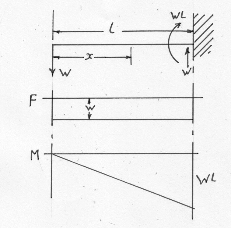
A Cantilever of length l carries a concentrated load W at its free end. Draw the Shear Force (SF) and Bending Moment (BM) diagrams.

Click to see Solution

Example 2

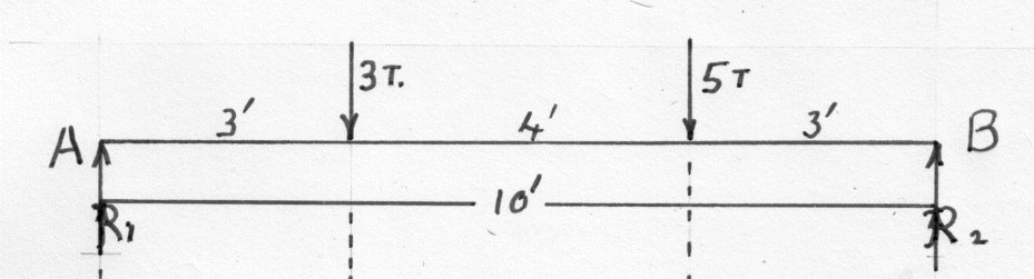
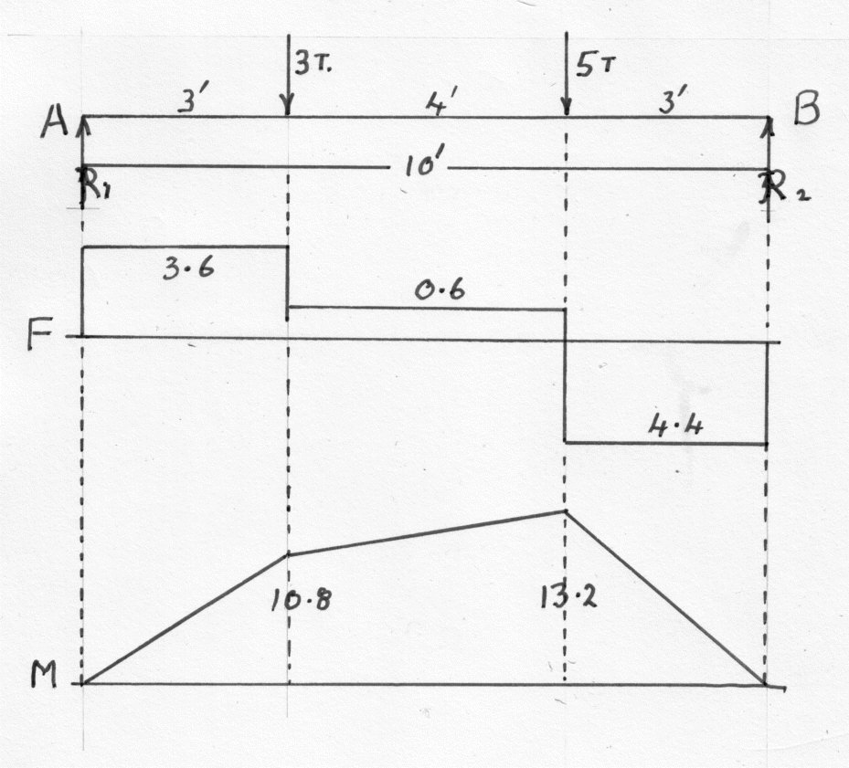
A beam 10 ft. long is simply supported at its ends and carries concentrated loads of 3 tons and 5 tons at distances of 3 ft. from each end. Draw the SF and BM diagrams.

Click to see Solution

Uniformly Distributed Loads

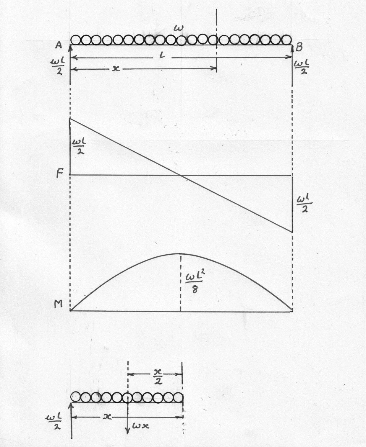
Example 3

Draw the SF and BM diagrams for a Simply supported beam of length l carrying a uniformly distributed load w per unit length which occurs across the whole Beam.

Click to see Solution

Combined Loads

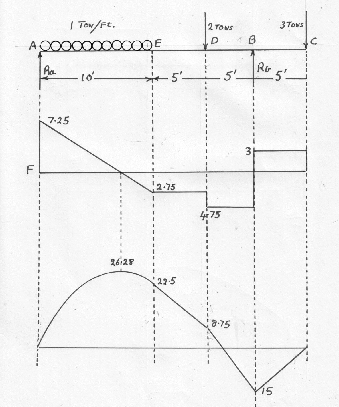
Example 4

A Beam 25 ft. long is supported at A and B and is loaded as shown. Sketch the SF and BM diagrams and find (a) the position and magnitude of the maximum Bending Moment and (b) the position of the point of contraflexure.

Click to see Solution

Example 5

A girder 30 ft. long carrying a uniformly distributed load of w ton/ft. is to be supported on two piers 18 ft. apart so that the greatest Bending Moment will be as small as possible. Find the distance of the piers from the ends of the girder and the Maximum B.M. (U.L.)

Let the distance of one pier be d ft.from the end of the girder. Hence the other overhang will be 12 - d.

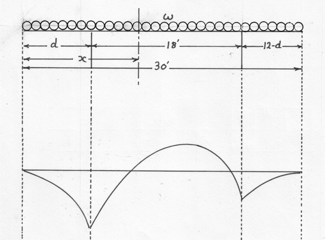
Taking Moments about the right-hand support. The distance of the centre of the girder from the right-hand support is (3 + d):-

$Hence\;\;\;\;\;\;\;18\,R\;=\;30\,w\,(3\;+\;d)$

(33)

$\therefore\;\;\;\;\;\;R\;=\;\left(\frac{5w}{3} \right)\left(3\;+\;d \right)$

(34)

For the overhanging end $\displaystyle M\;=\;-\,\frac{wx^2}{2}$ which gives a maximum value at the support of :-

$M\;=\;-\,\frac{wd^2}{2}$

(35)

For the portion between the supports:-

$M\;=\;-\,\frac{wx^2}{2}\;+\;R\left(x\;-\;d \right)$

(36)

This is a maximum when

$\frac{dM}{dx}\;=\;0\;=\;-wx\;+\;R$

(37)

Using this equation and equation (34):-

$x\;=\;\frac{R}{w}\;=\;\left(\frac{5}{3} \right)\left(3\;+\;d \right)$

(38)

$\therefore\;\;\;\;\;\hat{M}\;=\;-\,\left(\frac{25}{18}\right)w\left(3\;+\;d \right)^2\;+\;\left(\frac{5w}{3} \right)(3\;+\;d)\left\{\left(\frac{5}{3} \right)(3\;+\;d)\;-\;d \right\}$

(39)

$=\;-\;\left(\frac{25w}{18} \right)(3\;+\;d)^2\;+\;\left(\frac{5w}{9} \right)(3\;+\;d)(15\;+\;2d)$

(40)

$=\;\frac{5w}{18}(45\;+\;12d\;-\;d^2)$

(41)

For the greatest BM to be as small as possible is is necessary to make the two values numerically equal. It is clear that if the supports are moved to the right of this position the value at the left support will increase and if it is moved to the left the value between the supports will increase.

Equating the numerical values from equations (34) and (41)

$\frac{wd^2}{2}\;=\;\frac{5w}{18}(45\;+\;12d\;-5d^2)$

(42)

$\therefore\;\;\;\;\;9d^2\;=\;225\;+\;60d\;-\;5d^2$

(43)

$Or\;\;\;\;\;\;\;14d^2\;-\;60d\;-\;225\;=\;0$

(44)

Solving:-

$d\;=\;\frac{60\mp \sqrt{(3600\;+\;4\times14\times225)}}{28}\;=\;6.7ft\;\;\;\;\;(one\;support)$

(45)

And for the other support:-

$12\;-\;d\;=\;5.3ft.$

(46)

From equation (34)

$\hat{M}\;=\;\frac{wd^2}{2}\;\;\;\;\;\;(numerically)$

(47)

$22.4w\;tons-ft.$

(48)

Example 6

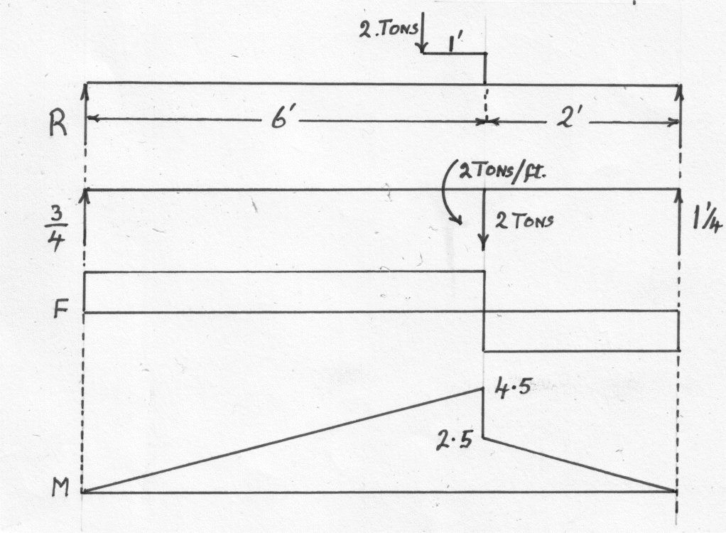
Draw the SF and BM diagrams for a beam 8 ft. long simply supported at its ends, carrying a load of 2 tons which is applied through a bracket. The bracket is fixed to the beam at a distance 0f 6ft. from one support, the length of bracket in the direction of the beam being 1 ft.

Blank

Taking Moments about the right hand end:-

$R\;=\;\frac{(2\times3)}{8}\;=\;\frac{3}{4}\,tons$

(49)

The effect of the bracket is to apply a load of 2 tons and a B.M. of 2 ton_t at a point 6 ft. from the left hand end.

Thus F has a value of 3/4 tons along 6 ft. of the beam from the left-hand end and $\displaystyle -\,1\frac{1}{4}\;tons$ fro the other two foot

M increases from zero to $\displaystyle \frac{3}{4}\times2\;=\;2.5\,tons-ft.$ at the bracket on the other side. There is a sudden change in Bending Moment at the bracket equal to 2 tons-ft.

Varying Distributed Loads.

Example 7

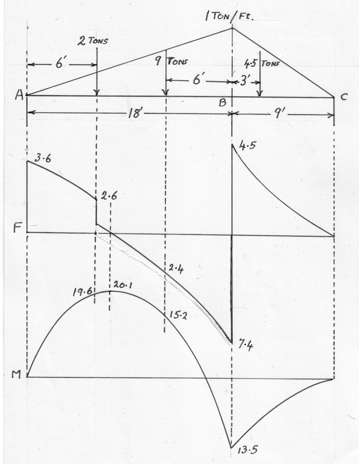
A Beam ABC, 27 ft. long, is simply supported at A and B 18 ft. across and carries a load of 2 tons at 6 ft. from A together with a distributed load whose intensity varies in linear fashion from zero at A and C to 1ton/ft. at B.

Draw the Shear Force and Bending Moment diagrams and calculate the position and magnitude of the maximum B.M. (U.L.)

The Total Load on the beam ( i.e. the load plus the mean rate of loading of 1/2 tons/ft) is given by:-

$Load\;=\;2\;+\;\frac{1}{2}\times27\;=\;15.5\,tons$

(50)

Blank

The Total distribute load on $\displaystyle AB\;=\;\frac{1}{2}\times18\;=\;9\;\;tons$ and on $\displaystyle BC\;=\;\frac{1}{2}\times9\;=\;4.5\;\;tons$ each of which act through their centres of gravity. These are $\displaystyle \frac{2}{3}\times 18\;=\;12\;\;ft.$ from A and $\displaystyle \frac{2}{3}\times 9\;=\;6\;\;ft.$ from C in the other case. (Note. These are the centroids of the triangles which represent the load distribution)

Taking Moments about B

$R_1\;=\;\left(\frac{2\times12\;+\;9\times6\;-4.5\times3}{18} \right)\;=\;3.6\;\;tons$

(51)

$\therefore\;\;\;\;\;R_2\;=\;2\;+\;9\;+\;4.5\;-\;3.6\;=\;11.9\;\;tons$

(52)

At a distance x (<18)from A the loading is x/18 tons/ft.. The Total distributed load on this length is:-

$(Mean\;rate\;of\;loading)\times x\;=\;\frac{1}{2}\left(\frac{x}{18} \right)\;x\;=\;\frac{x^2}{36}\;\;tons$

(53)

The centre of gravity of this load is $\displaystyle \frac{2}{3}\;x$ from A.

For 0<x<6

$F\;=\;3.6\;-\;\frac{x^2}{36}$

(54)

At x = 6 ft.

$F\;=\;2.6\;\;tons$

(55)

$M\;=\;3.6\,x\;-\;\left(\frac{x^2}{36} \right)\times \frac{x}{3}\;=\;3.6\,x\;-\;\frac{x^3}{108}$

(56)

At x = 6 ft.

$M\;=\;19.6\;\;tons-ft.$

(57)

6< x <18

$f\;=\;3.6\;-\;2\;-\;\frac{x^2}{36}$

(58)

$At\;x\;=\;12\;\;ft.\;\;\;\;\;\;\;\;F\;=\;-\;2.4\;\;tons$

(59)

$At\;x\;=\;18\;\;ft.\;\;\;\;\;\;\;\;F\;=\;-\;7.4\;\;tons$

(60)

$F\;=\;0\;\;\;\;when\;\;\;\;x\;=\;6\;\sqrt{1.6}\;=\;7.58\;ft.$

(61)

Blank

$M\;=\;3.6x\;-\;2(x\;-\;6)\;-\;\frac{x^3}{108}\;=\;1.6x\;+\;12\;-\;\frac{x^3}{108}$

(62)

$At\;x\;=\;12\;\;ft\;\;\;\;\;\;\;\;M\;=\;15.2\;\;tons-ft.$

(63)

$At\;x\;=\;12\;\;ft\;\;\;\;\;\;\;\;M\;=\;-\;13.5\;\;tons-ft.$

(64)

The maximum Bending Moment occurs at zero s earing force 1.e.x = 7.58 ft.

$\therefore\;\;\;\;\;\hat{M}\;=\;20.1\;\;tons-ft.$

(65)

The section BC can be more easily calculated by using a variable X measured from C. Then by a similar argument:-

$F\;=\;\frac{1}{2}\left(\frac{X}{9} \right)X\;=\;\frac{X^2}{18}\;\;tons$

(66)

$At\;\;\;X\;=\;9\;\;ft.\;\;\;\;\;\;\;\;F\;=\;4.5\;\;tons.$

(67)

$M\;=\;-\;\frac{1}{2}\left(\frac{X}{9} \right)X\left(\frac{X}{3} \right)\;=\[-\frac{X^3}{54}\;\;ton-ft.$

(68)

$At\;\;\;X\;=\;9\;\;ft.\;\;\;\;\;\;\;\;\;\;=-\;13.5\;\;tons-ft.$

(69)

The complete diagrams are shown. It can e seen that for a uniformly varying distributed load, the Shearing Force diagram consists of a series of parabolic curves and the Bending Moment diagram is made up of "cubic" discontinuities occurring at concentrated loads or reactions. It has been shown that Shearing Forces can be obtained by integrating the loading function and Bending Moment by integrating the Shearing Force, from which it follows that the curves produced will be of a successively "higher order" in x ( See equations (6) and(7))

Graphical Solutions

Note This method may appear complicated but whilst the proof and explanation is fairly detailed, the application is simple and straight forward.

Earlier it was shown that the change of Bending Moment is given by the double Integral of the rate of loading. This integration can be carried out by means of a funicular polygon. See diagram.

Suppose that the loads carried on a simply supported beam are $\displaystyle W_1; W_2; W_3;\;and\;W_4\;and\;that\; R_1\;and\;R_2$ are the reactions at the supports. Letter the spaces between the loads and reactions A; B; C; D; E; and F.

Draw to scale a vertical line such that $\displaystyle a\,b\;=\;W_1;\;\;\;b\,c\;=\;W_2;\;\;\;c\,d\;=\;W_3;\;\;\;and\;\;\;d\,e\;=\;W_4$ . Now take any point "O" to the left of the line and join O to a; b; c; d; and e. This is called The Polar Diagram

Commencing at any point p on the line of action of $\displaystyle R_1$ draw pq parallel to Oa in the space "A" , qr parallel to Ob in the space "B" and similarly rs; st; and tu. Draw Of parallel to pu.

It will now be shown that fa represents $\displaystyle R_1$ . Also pqrstu is the Bending Moment diagram drawn on a base pu, M being proportional to the vertical ordinates.

$\displaystyle W_1$ is represent by ab and acts through the point q; it can be replaced by forces aO along qp and Ob along qr. Similarly $\displaystyle W_2$ can be replaced by forces represented by bO along rq and Oc along rs; $\displaystyle W_3$ by cO along sr and Od along st etc.

All of these forces cancel each other out except aO along qp and Od along te and these two forces must be in equilibrium with $\displaystyle R_1\;and\;R_2$ . Tis can only be so if $\displaystyle R_1$ is equivalent to a force Oa along pq and fO along up, $\displaystyle R_2$ being equivalent to eO along ut and Of along pu. Hence $\displaystyle R_1$ is represented by fa and $\displaystyle R_2$ by ef.

Blank

Blank

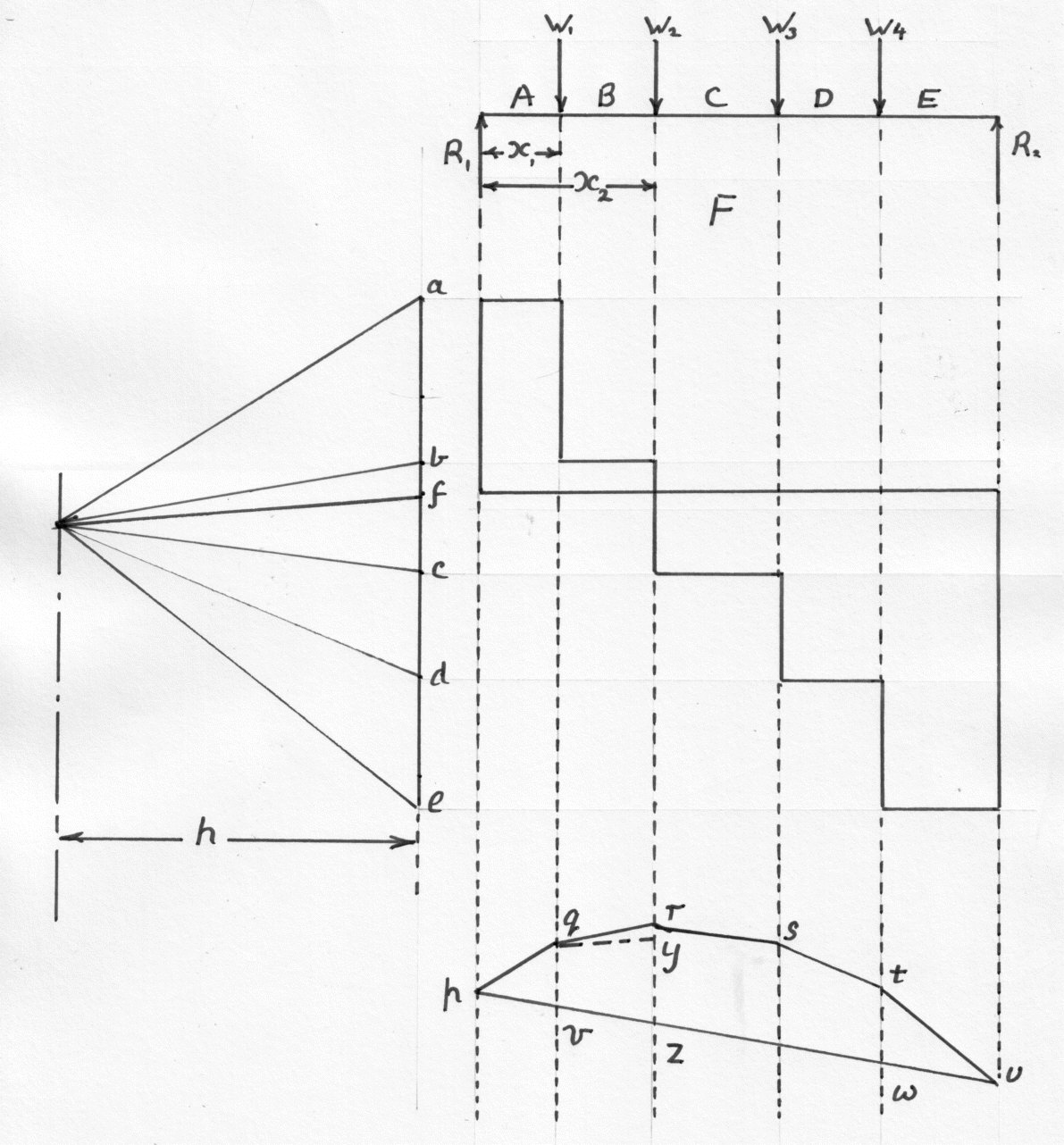
triangles pqv and Oaf are similar and hence:-

$q\,v\;=\;af.\frac{pv}{Of}$

(70)

$Or\;\;\;\;\;qv\propto a\,f\;\frac{x_1}{h}$

(71)

Where $\displaystyle x_1$ is the distance from $\displaystyle W_1$ from the left-hand end of the beam and h is the length of the perpendicular from O on to ae.

But $\displaystyle ay\,.\,x_1\;\propto \;R_1\,x_1\;\;\;\;i.e.\;the\;BM\;at\;x_1$

Hence for a given position of the pole O, qv represents the B>M> at $\displaystyle x_1$ to a certain scale.

If qy is drawn parallel tp pu, then the triangle qry is similar to Obf and:-

$r\,y\;=\;b\,f\left(\frac{qy}{of} \right)\;=\;b\,f\left( \frac{x_2\;-\;x_1}{h}\right)$

(72)

$\therefore\;\;\;\;\;rz\;=\;qv\;+\;ry\;=\;af\,\left(\frac{x_1}{h} \right)\;+\;bf\left(\frac{x_2\;-x_1}{h} \right)$

(73)

$which\;is\;\propto R_1x_1\;=\;(R_1\;-\;W_1)(x_2\;-\;x_1)\;=\;R_1x_2\;-\;W_1(x_2\;-X_1)$

(74)

Which is the Bending Moment at $\displaystyle x_2$ .

Similarly the ordinates at the other load points give the Bending Moments at those points, the scale being determined as follows:-

If the load scale of the Polar Diagram is $\displaystyle 1\;in.\;=\;s_1\;lb.,$ then the length scale along the beam is $\displaystyle 1\;in.\;=\;s_2\;ft.,$ and the Bending Moment scale required is $\displaystyle 1\;in.\;=\;s_3\;lb.ft.,$ then the length

$\displaystyle qv\propto af.\frac{x_1}{h}$ as shown above

$=\;\frac{W_1x_1}{s_1s_2h}\;=\;\frac{M}{s_1s_2h}$

(75)

$But\;\;\;\;\;qv\;=\;\frac{M}{s_3}$

(76)

$\therefore\;\;\;\;\;h\;=\;\frac{s_3}{s_2s_2}\;in.$

(77)

If a base on the same level as f is drawn and the points a, b, c, d, and e are projected across from the Polar Diagram, then the Shearing Force diagram is obtained.

This method can be equally well used for distributed loads bby dividing the loading daigram into strips and taking the load on a strip to act as if it were concentrated at its centre og gravity.

For cantilevers, if the Pole O is taken on the same horizontal level as the point a then the base of the Bending Moment will be horizontal.

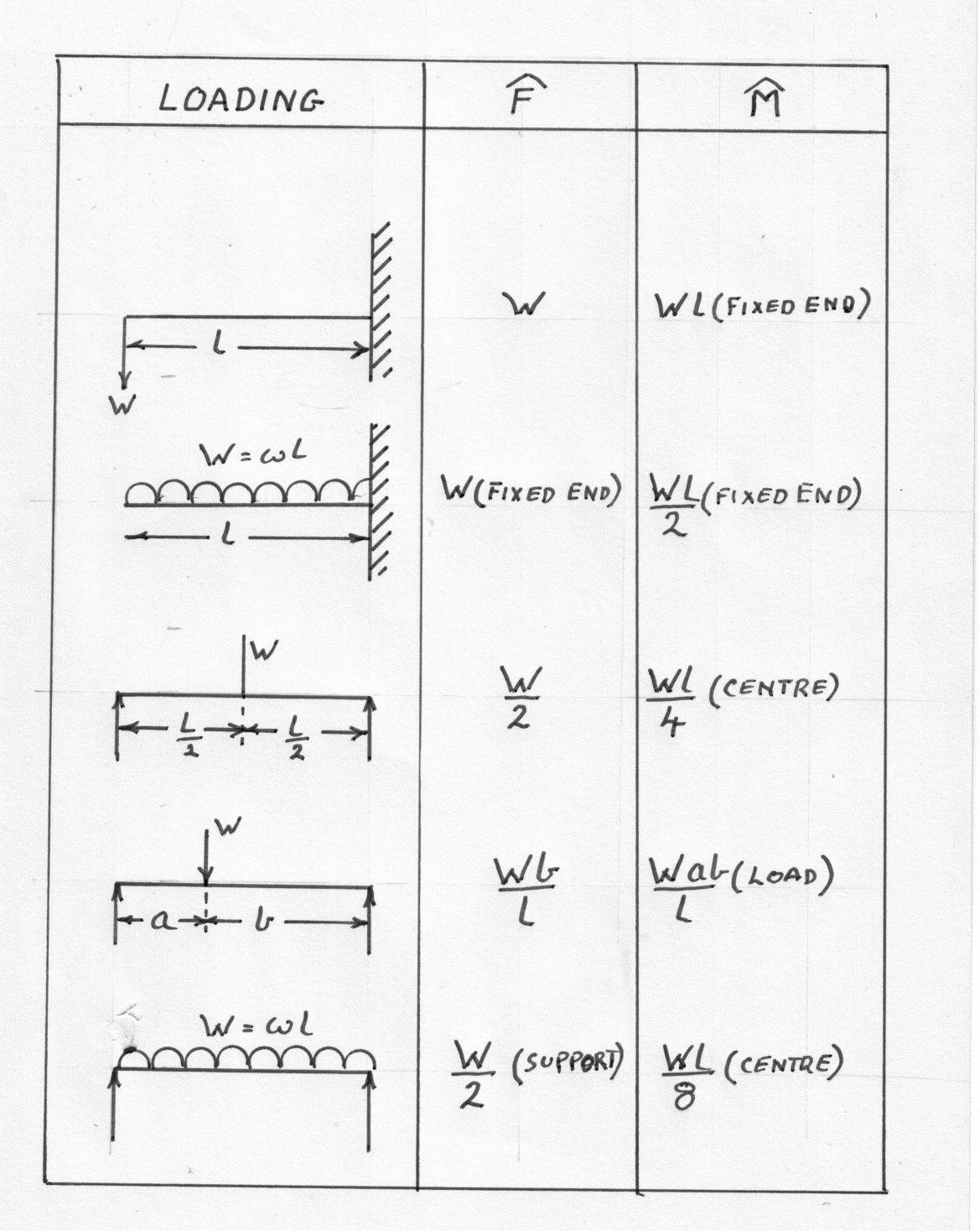
Appendix

Shearing Force F

Mending Moment M

Rate of loading w

$F\;=\;\frac{dM}{dx}$

(78)

$w\;=\;-\,\frac{dF}{dx}\;=\;-\frac{d^2M}{dx^2}$

(79)

Blank