Branched Pipes

Bernoulli's principle states that for an inviscid flow, an increase in the speed of the fluid occurs simultaneously with a decrease in pressure or a decrease in the fluid's potential energy. Bernoulli's principle can be applied to various types of fluid flow, resulting in what is loosely denoted as Bernoulli's equation.

The application of the Bernoulli's equation to Branched pipes.

You're viewing an older version of this page (#3976). View the current version.

View versions (5)

Introduction

It is common for a pipeline to be branched and for the system to be feeding more than one reservoir. A similar arrangement is seen in a combination of three or more pipes joining as many reservoirs, meeting at a common junction. This page examines these conditions using the Bernoulli's equation.

Branched Pipes

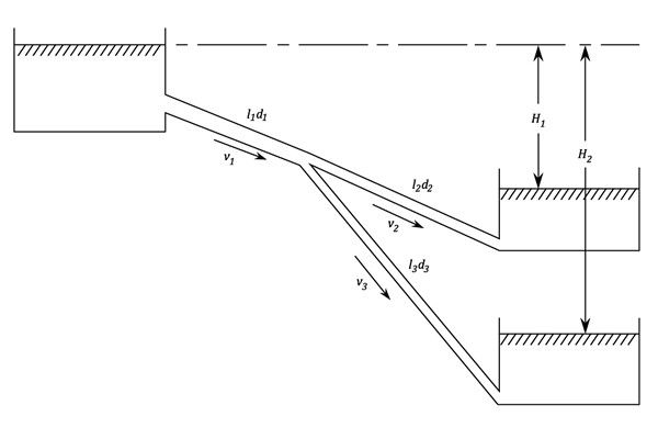
Applying Bernoulli's equation to the whole system but neglecting both the entry head and the junction head.

$H_1=\frac{4fl_1{v_{1}}^{2}}{2d_1g}+\frac{4fl_2{v_{2}}^{2}}{2d_2g}+\frac{{v_{2}}^{2}}{2g}$ $H_2=\frac{4fl_1{v_{1}}^{2}}{2d_1g}+\frac{4fl_3{v_{3}}^{2}}{2d_3 g}+\frac{{v_{2}}^{2}}{2g}$

It most cases it is possible to neglect the last terms of $\displaystyle\frac{v^2}{2g}$ .

Applying the continuity equation: $a_1v_1=a_2v_2+a_3v_3$ or ${d_{1}}^{2}v_1={d_{2}}^{2}2v_2+{d_{3}}^{2}v_3$

Example 1

Problem

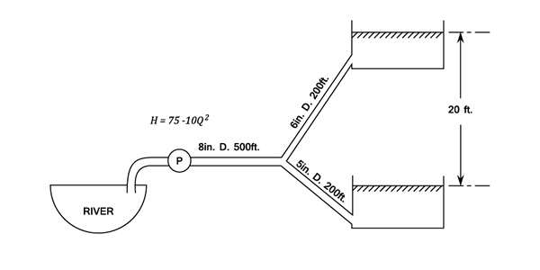
Water is pumped from a river to two reservoirs $A$ and $B$ . The water surface in reservoir $A$ is at the same hight as the river whilst that in reservoir $B$ is 20 ft. higher.

Pumping from the river takes place by means of a centrifugal pump, the equation relating flow $Q$ (in cubic ft./sec.) and $H$ ft. at a constant speed being given by $H=75-10\;Q^2$

From the river to a junction $J$ is a common pipe is used of 8 in. diameter and 500 ft. long. The branch $J$ to the reservoir $A$ is 5 in. in diameter and 200 ft. long. The branch from $J$ to reservoir $B$ is 6 in. in diameter and 200 ft. long.

Neglecting all losses other than pipe friction, calculate the discharge to $A$ and $B$ . Take $f$ as 0.007 throughout.

Workings

Darcy's equation can be rewritten as follows:

$h_f=\frac{4flv^2}{2dg}=\frac{flQ^2}{10d^5}$

Applying Bernoulli at the river and reservoir $A$ :

$H=\frac{0.007\times 5000\times Q^2}{10\times \left ( \tfrac{8}{12} \right )^5}+\frac{0.007\times 2000\times {Q_{A}}^{2}}{10\times \left ( \tfrac{5}{12} \right )^5}=75-10\;Q^2$

$\therefore \;\;\;\;\;\;26.57Q^2+111.5{Q_{A}}^{2}=75-10Q^2$

(1)

Similarly: $H-20=\frac{0.007\times 5000\times Q^2}{10\times \left ( \tfrac{8}{12} \right )^5}+\frac{0.007\times 2000\times {Q_{B}}^{2}}{10\times \left ( \tfrac{6}{12} \right )^5}=75-10\;Q^2-20$

$\therefore \;\;\;\;\;\;26.57Q^2+44.8{Q_{A}}^{2}=55-10Q^2$

(2)

But by continuity:

$Q=Q_A+Q_B$

(3)

From equation (#1)

$Q^2=2.05-3.05{Q_{A}}^{2}$

(4)

Subtracting equation (#2) from (#1) $111.5{Q_{A}}^{2}-44.8{Q_{B}}^{2}=20$ $\therefore \;\;\;\;\;\;{Q_{A}}^{2}=2.49{Q_{B}}^{2}-0.446$

Substituting into equation (#3) squared with values for $Q$ from equation (#4) gives: $2.05-3.05{Q_{A}}^{2}={Q_{A}}^{2}+2.49{Q_{A}}^{2}-0.446+20A\;\sqrt{2.49{Q_{A}}^{2}-0.446}$