CodeCogs

The selection of Specific Speed and Unit Conditions for turbines with reference to Model Testing

You're viewing an older version of this page (#3591). View the current version.

Introduction

In the selection and or design of turbines for a particular application it is common to rely on model testing. The results are then scaled up using the following principles

Principles of Similarity Applied to Turbines.

( The figures used in this section are based on the ft.; slug ; Second . system)

A similar model means :-

Geometrically similar - made from the same drawings but to a different scale.
Dynamically similar - Operating conditions and equal efficiencies.

Thus in comparing two similar turbines

All the linear dimensions will be in the same ratio.
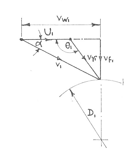
All angles will be the same; the velocity triangles will be geometrically similar and all velocities will be in the same ratio.

Specific speed of a turbine

The Specific Speed $N_s$ of a turbine is the speed in r.p.m. at which a similar model of the Turbine would run under a head of 1ft. when of such a size as to develop 1 H.P. Note The suffix "s" is used to denote the values associated with the Specific Turbine)

Each type of Turbine (Pelton Wheel; Francis etc.) has it's own characteristic limits of $n_s$ .

$\text{But}\;\;\;\;\;\; V = K\sqrt{2gH}$

(1)

$\therefore\;\;\;\;\;v\propto V_f\propto V\propto \sqrt{H}$

(2)

$\text{and}\;\;\;\;\;v = \frac{\pi D\,N}{60}$

(3)

$\therefore\;\;\;\;\;D\;\propto \frac{\sqrt{H}}{D}$

(4)

But Q = The Area of flow X the Velocity of flow

$Q = K\,\pi \;D\;b\;V_f\;\;\;\;\;\;\;\text{and}\;\;\;\;b\;\propto D$

(5)

$\text{or}\;\;\;\;\;Q\;\propto \;D^2\;\sqrt{H}$

(6)

$\text{But the weight of water per second}\;\;W=w\times Q\;\;\;\;\text{Which is}\propto \frac{H^\frac{3}{2}}{N^2}$

(7)

$\therefore \text{ H.P.output of the Turbine}\;\;P=\frac{W\times H}{550}\times \eta\;\;\;\;\text{Which is}\;\;\propto \frac{H^\frac{5}{2}}{N^2}$

(8)

Note The efficiencies are equal

$\therefore\;\;\;\;\;\frac{N\;\sqrt{P}}{H^{\frac{5}{4}}} = \text{Constant} = \frac{N_s\,\sqrt{P_s}}{H_s^{\frac{5}{4}}}$

(9)

$\text{But for the specific Turbine} \;P_s\;\text{and}\;H_s\;are 1$

(10)

$\therefore\;\;\;\;\;N_s = \frac{N\;\sqrt{P}}{H^{\frac{5}{4}}}$

(11)

Notes on the use of the Specific Speed of a Turbine

$N_s$ is based on the values of N; P; and H used at the design point. i.e. At maximum efficiency.
$N_s$ is NOT dimensionless and there are different values in each of the measurement systems.

Unless otherwise stated, N is in r.p.m.and P is in Brake Horse Power(b.h.p.) i.e. $\displaystyle \frac{ft.lb./sec}{550}$

The Dimensions of Specific Speed

$\text{The unit of} N_s\text{ are}}\; \frac{1}{T}\left(\frac{LM}{T^2}\frac{L}{T} \right)}^{\frac{1}{2}}\div L^{\frac{5}{4}}$

(12)

$=\frac{M^\frac{1}{2}}{T^\frac{5}{2}\;L^\frac{1}{4}}$

(13)

The Speed Number

$N_s$ can be made dimensionless and still be a constant by dividing by $w^\frac{1}{2}\;g^\frac{3}{4}$ and this is called the The Speed Number

The Specific Speed of a Particular form of Turbine

For a particular type of Turbine $N_s$ is constant.

$v = \frac{\pi \,D\,N}{60}\;\;\;\;and\;\;\;\;v\propto \sqrt{H}$

(14)

$\therefore\;\;\;\;\;N\propto \sqrt{H}\;\;\;\;or\;\;\;\;\frac{N}{\sqrt{H}}\;\text{which is constant}$

(15)

But

$P = \frac{W\;H}{550}\times \;\text{efficiency}\;\;\propto W\;H\;\;\propto \;w\;Q\;H\;\propto D^2\:V_f\H\;\propto H^\frac{3}{2}$

(16)

$\therefore\;\;\;\;\;\frac{P}{H^\frac{3}{2}} = \text{Constant}$

(17)

$\therefore\;\;\;\;\;\sqrt{\frac{P}{H^\frac{3}{2}}}\times \frac{N}{\sqrt{H}} = \frac{N\sqrt{P}}{H^\frac{5}{4}}=\text{Constant} = N_s$

(18)

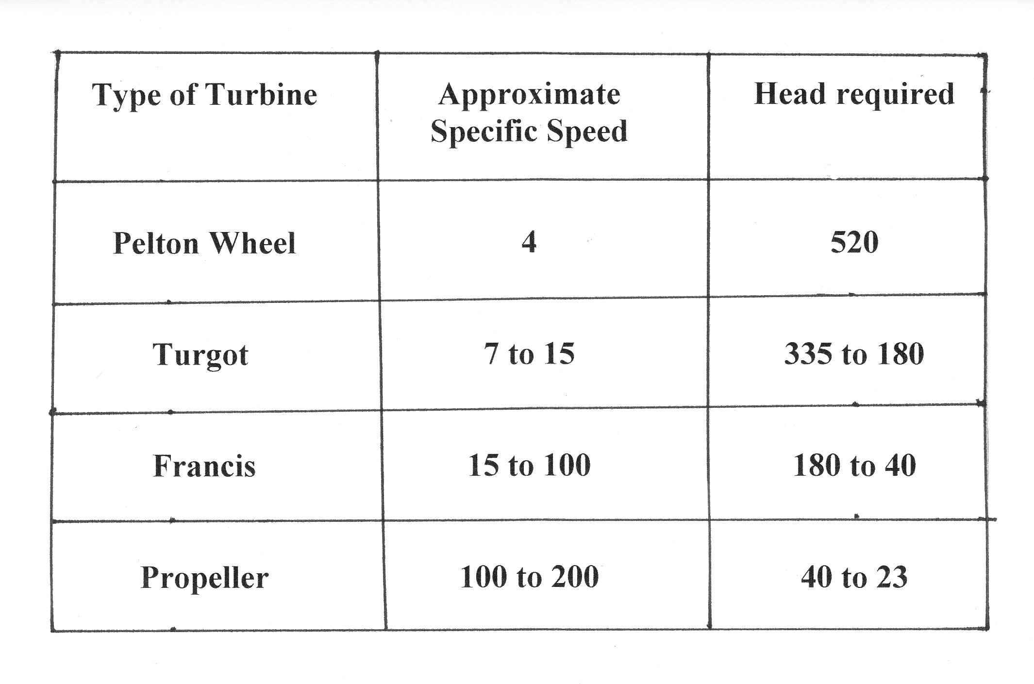
Specific Speeds for Differing types of Turbine

For different types of Turbine $N_s$ and a comparison of heads for a particular power and speed. The Turbine is required to develope100 b.h.p. at 1000 r.p.m.

An example of the use of Specific Speed.

What type of turbine would be used if the supply head is of 10 cu.ft/sec with a head of 225 ft. ? Assume an efficiency of 80%.

Power Output = Water h.p.input X Efficiency

$= \frac{0.8\;w\;Q\,H}{550}$

(19)

$= \frac{0.8\times 62.4\times 10\times 225}{550} = 204\;h.p.$

(20)

$N_s = \frac{N\sqrt{P}}{H^\frac{5}{4}} = \frac{600\sqrt{204}}{225^\frac{5}{4}} = 9.83$

(21)

It would therefore be necessary to use a Turgot Turbine. However it might be possible to use a Pelton Wheel with two jets.

$\text{Power per jet}\; = \frac{204}{2}h.p.$

(22)

$\therefore\;\;\;\;\;N_s\text{per Jet} = \frac{9.83}{\sqrt{2}} = 6.95$

(23)

From the above table it can be seen that the value of $N_S$ is too high. It is therefore worth considering a Pelton Wheel with four jets.

$\text{Now}\;\;\;\;\;N_s \text{per Jet} = \frac{9.83}{\sqrt{4}} = 4.92$

(24)

This would be a practical proposition but would result in some loss of efficiency due to interference between the jets. Consequently a better alternative would be to have two wheels on the same shaft with two jets per wheel.

Unit Conditions

The unit operating conditions for a turbine are those under which that particular turbine would run when working under a head of one ft. ( or unit head in any other system) assuming there to be no change in efficiency. This allows the performance of a given turbine to be compared when working under different heads and enables the characteristic curves to be drawn which show the efficiency at all running conditions.

Unit Speed

If $N_u$ is the Unit speed and N the speed under a head H

$v = \frac{\pi DN}{60}\;\;\;\;\;\text{and}\;\;\;v\propto V \propto H$

(25)

$\therefore\;\;\;\;\;N \propto \sqrt{H}$

(26)

$\frac{N}{\sqrt{H}}=\text{constant}=\frac{N_u}{\sqrt{H_u}} \;\;\;\text{Where u represents unit conditions}$

(27)

$\therefore\;\;\;\;\;\text{Unit speed}\;N_u=\frac{N}{\sqrt{H}}$

(28)

Unit Quantity

The Unit quantity of a Turbine is the flow through the turbine when operating under a head of one ft. assuming similar conditions. Let:-

Q be the flow under a head H
Therefore Q is the area of flow X velocity

And since the area is constant and the velocity is $\propto \;\sqrt{H}$

$Q\propto \sqrt{H}\;\;\;\;\text{or}\;\;\;\;\frac{Q}{\sqrt{H}} = \text{Constant}$

(29)

$\therefore\;\;\;\;\;\frac{Q}{\sqrt{H}} = \frac{Q_u}{\sqrt{H_u}}$

(30)

Unit Power

The Unit Power of a given turbine is the power output of the turbine when operating under a head of one ft. assuming no change in efficiency . If P is the output under a head H

$\text{Then}\;\;\;\;\;P = \frac{W\;H}{550}\times \eta$

(31)

$\text{If}\;\eta \;\text{is unchanged}\;W = w \;Q \;\text{And if}\;\eta \;\text{is unchanged}\;W = w\,Q$

(32)

$\therefore\;\;\;\;\;W\propto \sqrt{H}\;\;\;and\;\;\;P\propto \sqrt{H}\times H\;\;\;\;\propto H^{\frac{3}{2}}$

(33)

$\therefore\;\;\;\;\;\frac{P}{H^{\frac{3}{2}}} = \text{Constant} = \frac{P_u}{H_u^{\frac{3}{2}}}$

(34)

But $H_u = 1$

$\therefore\;\;\;\;\;\text{Unit Power}\;P_u = \frac{P}{H^{\frac{3}{2}}}$

(35)

$\text{Note}\;\;\;\;N_u\sqrt{P_U} = \frac{N}{\sqrt{H}}\times \frac{\sqrt{P}}{H^{\frac{3}{2}}} = \frac{N\sqrt{P}}{H^{\frac{5}{4}}} = N_s$

(36)

The Performance Curves of a Turbine

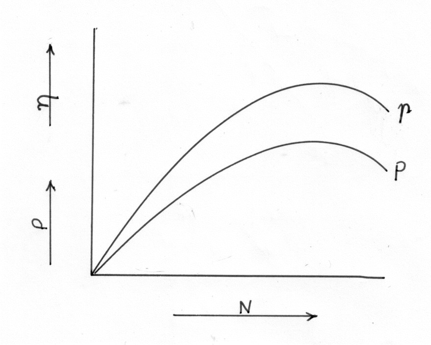
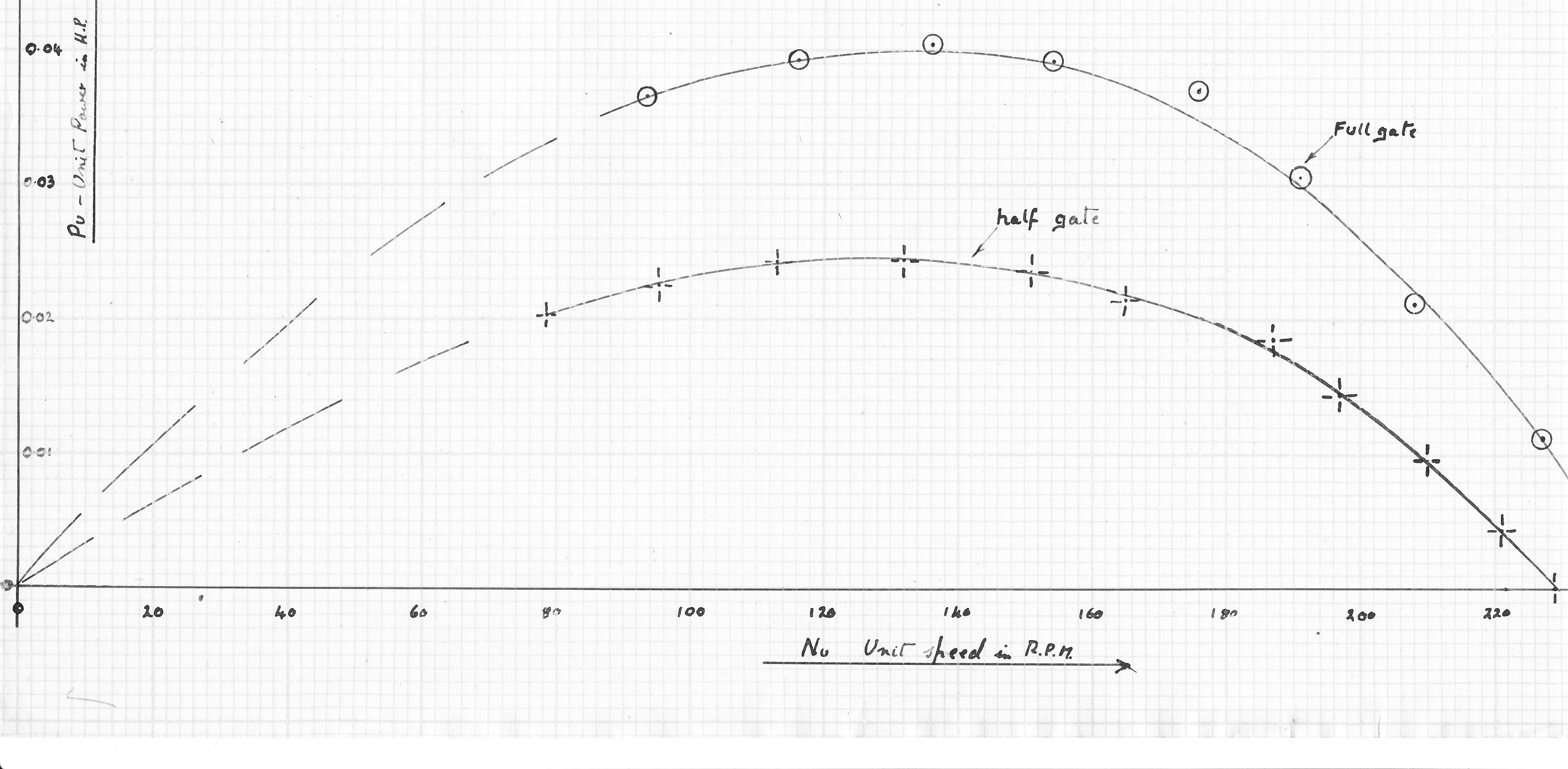
Performance Curves are plotted for a constant head and a constant Gate opening ( Or needle valve setting) and are on the basis of speed in r.p.m.

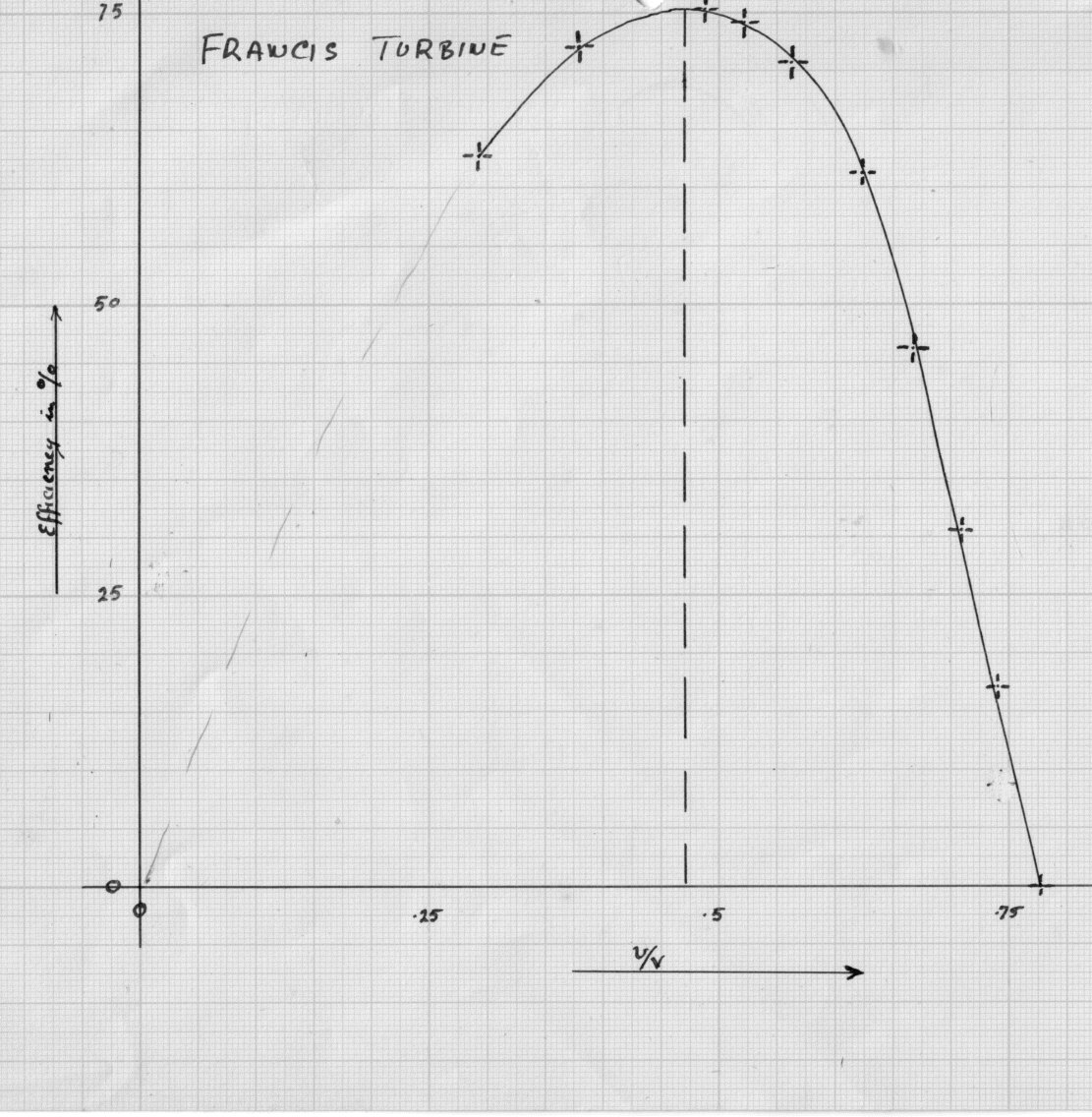
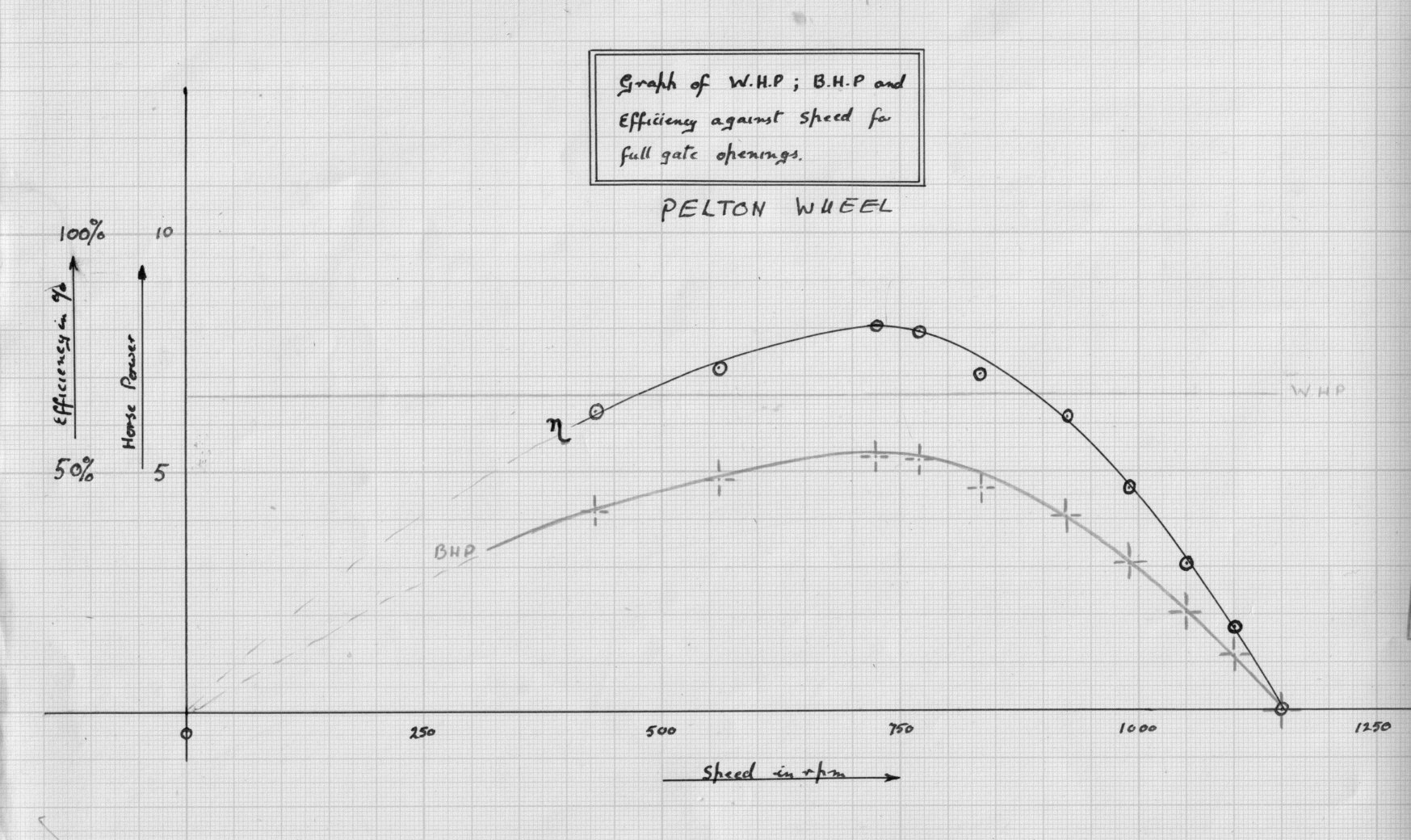
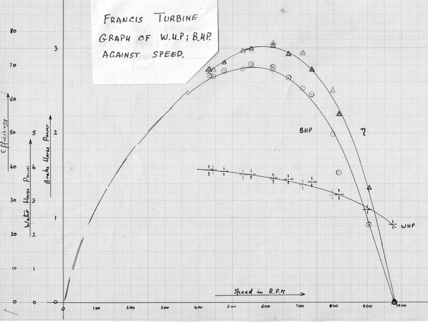
Characteristic curves and iso-efficiency curves for a turbine under all operating conditions

The Turbine is tested under a constant head H for each of several gate openings and the values of Power output P and speed N are reduced to unit conditions ( Equations (125) (132)). Suitable values for efficiency are the marked on the curve for the differing Gate openings and lines of iso-efficiency are drawn.

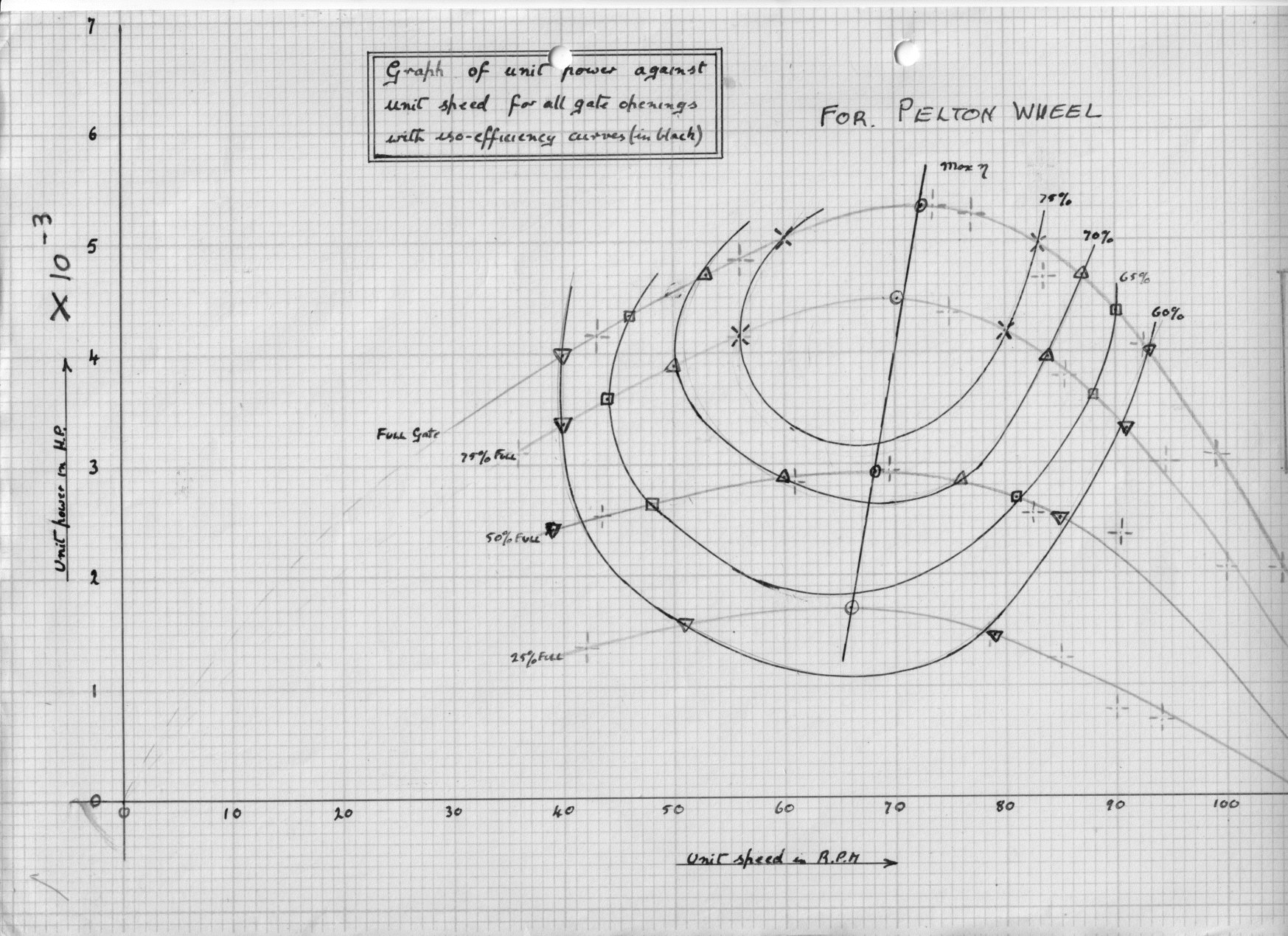
These graphs enable the best running speed or the best gate opening to be chosen and the corresponding power output for that speed and gate setting to be found for any particular head.

An example of the use of unit conditions

A Francis Turbine develops 3240 h.p. at 120 rpm when under a head of 36 ft. What would be the speed and output under a head of 25 ft. assuming no loss in efficiency.

$N_u = \frac{N}{\sqrt{H}} = \frac{N_1}{\sqrt{H_1}}$

(37)

$\therefore\;\;\;\;\;\frac{120}{\sqrt{36}} = \frac{N_1}{\sqrt{25}}$

(38)

$\therefore\;\;\;\;\;N_1 = 100\,r.p.m.$

(39)

But since $H_u=1$

$Q_u = \frac{Q}{\sqrt{H}}$

(40)

$\text{Unit Power}\;P_u = \frac{P}{H^\frac{3}{2}} = \frac{P_1}{H_1^\frac{3}{2}} = \frac{3240}{36^\frac{3}{2}} = \frac{P_1}{25^\frac{3}{2}}$

(41)

$\therefore\;\;\;\;\;P_1 = 1875\; h.p.$

(42)

Fundamental Similarity Conditions and Model Testing

The following theory assumes equal efficiencies for both the Model and the Prototype. For geometrically similar turbines operating under dynamically similar conditions, the velocity triangles will be similar and:-

$v\propto V_f\propto V\propto \sqrt{H}$

(43)

but

$v = \frac{\pi DN}{60}$

(44)

$\therefore\;\;\;\;\;\sqrt{H} = DN\;\;\;\;or\;\;\;\;\frac{\sqrt{H}}{DN} = Constant}$

(45)

And

$Q = K\pi DbV_f\;\;\;\;\&\;\;\;\;b\propto D$

(46)

$\therefore\;\;\;\;\;Q\propto D^2\sqrt{H}\;\;\;\;or\;\;\;\;\frac{Q}{D^2\sqrt{H}} = \text{Constant\}] Substitute for H in the above equation. \[\therefore\;\;\;\;\;Q\propto ND^3\;\;\;or\;\;\;\frac{Q}{DN^3} = \text{Constant}$

(47)

Or substitute for D.

$Q\propto \frac{H}{N^2}\sqrt{H}\;\;\;\;or\;\;\;\;\frac{QN^2}{H^\frac{3}{2}} = \text{Constant}$

(48)

$\text{Power}\;\;P = \frac{WH}{550}\times \eta \;\;\;\text{if}\;\eta \;\text{is unchanged}\;\;\;P\propto QH$

(49)

From equation (146)

$P\propto D^2H^\frac{3}{2}\;\;\;\;or\;\;\;\;\frac{P}{D^2H^\frac{3}{2}} = \text{Constant}$

(50)

From Equation (148)

$P\propto \frac{H^\frac{3}{2}}{N^2}\times H\;\;\;\;or\;\;\;\;\frac{PN^2}{H^\frac{5}{2}} = \text{Constant}$

(51)

i.e.

$\frac{N\sqrt{P}}{H^\frac{5}{4}} = N_s = \text{Constant}$

(52)

From equations (144) and (150)

$P\propto D^2\propto D^3N^3\;\;\;\;or\;\;\;\;\frac{P}{N^3D^5} = \text{Constant}$

(53)

These seven expressions allow the performance of the prototype turbine to be estimated from tests on the model. Note that there are in fact only three independent equations.

The efficiency predicted for a large Turbine from test carried out on a model are usual lower than that obtained from the actual prototype. This is because of the relatively greater frictional losses in the smaller passages of the model.

Strictly speaking the surface finish of the model should be geometrically similar to that of the prototype. The reduction in efficiency is said to be due to scale effects and is correcter for in practice by the use of empirical equations such as The Moody equation.

$\frac{1 - \eta _p}{1 - \eta _m} = \left(\frac{D_m}{D_p} \right)^\frac{1}{4}\left(\frac{H_m}{H_p} \right)^\frac{1}{10}$

(54)

Example 1

A quarter scale Turbine is tested under a head of 36 ft.The full scale Turbine is required to work under a head of 100 ft.and to run at 428 r.p.m. At what speed must the model be run and if it develops 135 h.p. and uses 38cu.ft.of water per second at this speed, what power will be obtained from the full scale Turbine, assuming that it's efficiency is 3% better than that of the model.

$\left(\frac{\sqrt{H}}{ND} \right)_m = \left(\frac{\sqrt{H}}{ND} \right)_p$

(55)

$\therefore\;\;\;\;\;\frac{N_m}{N_p} = \sqrt{\frac{H_m}{H_p}}\times \frac{D_p}{D_m} = \sqrt{\frac{36}{100}}\times 4 = \frac{24}{10}$

(56)

$\therefore\;\;\;\;\;N_m = 2.4\times 428 = 1027\;r.p.m.$

(57)

$\text{W.H.P. of the model}\; = \frac{62.4\times 38\times 36}{550} = 155\;h.p.$

(58)

$\therefore\;\;\;\;\;\eta _m = \left(\frac{P_m}{W.H.P.} \right) = \frac{135}{155} = 87.1\%$

(59)

$\therefore\;\;\;\;\;\eta _p = 90.1\%$

(60)

But

$\left(\frac{Q}{ND^3} \right)_m = \left(\frac{Q}{ND^3} \right)_p$

(61)

$\frac{(WHP)_p}{(WHP)_m} = \frac{Q_p\,H_p}{Q_m\,H_m} = \frac{N_pD_p^3}{N_mD_m^3}\times \frac{H_p}{H_m} = \frac{10}{24}\times 4^3\times \frac{100}{36}$

(62)

$= \frac{2000}{27}$

(63)

$\therefore\;\;\;\;\;(WHP)_p = \frac{2000}{27}\times 155 = 11,500\;h.p.$

(64)

$= 1150\times 0.901 = 10,360\;h.p.$

(65)

$N_s = \frac{N\sqrt{P}}{H^\frac{5}{4}} = \frac{428\sqrt{10.360}}{100^\frac{5}{4}} = 138$

(66)

Blank

With a value for $N_s$ of 138 the Turbine must be a Propeller Turbine.

Example 2

An inward flow Reaction Turbine operating under an available head of H ft. of water, has a Specific Speed $N_S$ when the overall efficiency is $\eta$ per cent. If the water peripheral speed of the wheel is $k_1\sqrt{(2gH)}$ and the width of the wheel at its periphery is $k_2$ of the diameter, prove that the radial velocity of flow at entrance is given by:-

$v_{f1}=C\sqrt{2gH}\;\;\;\;\text{Where}\;\;\;\;C=\frac{{N_{s}}^{2}}{67190\;{k_{1}}^{2}k_2\eta}$

(67)

Hence find the guide blade angle and the vane angle at entrance to the wheel when $N_S=15$ $\eta=82.3\%$ $k_1=0.59$ $k_2=0.1$ and the hydraulic efficiency = 86.5% if the discharge is radial.

Blank

To see the solution please click on the red button