
Stiefel
Approximates a given function using the Stiefel-Remes method.
You're viewing an older version of this page (#280). View the current version.
Interface
#include <codecogs/maths/approximation/regression/stiefel.h>
using namespace Maths::Approximation::Regression;
Overview
This algorithm gives the best approximation of a continuous function with real argument in the sense of maximum norm. It uses the Stiefel-Remes method.
An important detail when using this class is that the abscissas array given as argument to the constructor needs to be sorted in ascending order and its elements need to be equally spaced, meaning that:
where N is the size of the array. In other words, the associated function needs to be discrete.
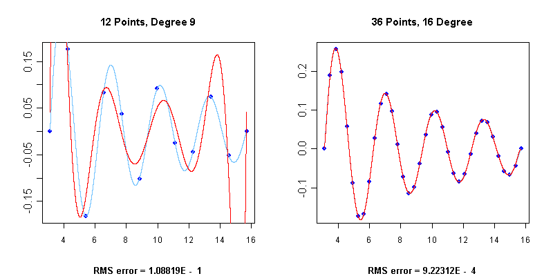
Below you will find the regression graphs for a set of points obtained by evaluating the function , displayed in light blue, at particular abscissas. The Stiefel-Remes polynomial, displayed in red, has been calculated using this class. In the first graph there had been chosen a number of 12 points and degree of polynomial 9, while in the second 36 points were considered with the polynomial degree 16. You may notice the root mean squared error in each of the cases.
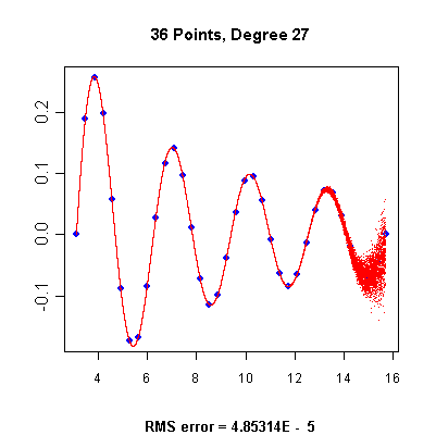
Choosing too high a degree, numerical rounding errors lead to high-frequency contamination of the results, which become increasingly evident with large values of x. This is visible with the following graph.
References
- "Procedures Algol en Analyse Numerique", Editions du CNRS, 1967
Example 1
#include <codecogs/maths/regression/stiefel.h>

#include <cmath>
#include <iostream>
#include <iomanip>
using namespace std;

#define PI  3.1415
#define N   12

int main()
{
    // Declare and initialize two arrays to hold the coordinates of the initial data points
    double x[N], y[N];

    // Generate the points
    double xx = PI, step = 4 * PI / (N - 1);
    for (int i = 0; i < N; ++i, xx += step) {
        x[i] = xx;
        y[i] = sin(2 * xx) / xx;
    }

    // Initialize the Stiefel-Remes approximation routine with known data points
    Maths::Regression::Stiefel A(N, x, y, 7);

    // Interrogate Stiefel polynomial to find approximated values
    int N_out = 20;
    xx = PI, step = (3 * PI) / (N_out - 1);
    for (int i = 0; i < N_out; ++i, xx += step)
        cout << "x = " << setw(7) << xx << "  y = " << setw(13) << A.getValue(xx) << endl;
    return 0;
}
Output:
x =  3.1415  y =       0.11495
x = 3.63753  y =      0.154609
x = 4.13355  y =     0.0875854
x = 4.62958  y =    0.00476885
x = 5.12561  y =    -0.0516197
x = 5.62163  y =    -0.0705339
x = 6.11766  y =     -0.058554
x = 6.61368  y =    -0.0298593
x = 7.10971  y =   0.000714345
x = 7.60574  y =     0.0219604
x = 8.10176  y =     0.0283645
x = 8.59779  y =     0.0203744
x = 9.09382  y =    0.00330991
x = 9.58984  y =    -0.0146569
x = 10.0859  y =    -0.0250193
x = 10.5819  y =    -0.0215192
x = 11.0779  y =   -0.00236588
x = 11.5739  y =      0.028343
x =   12.07  y =     0.0604278
x = 12.566 y = 0.079094Vince Cole (August 2005)
Members of Stiefel
CLASS METHOD
Stiefel
Initializes the necessary data for following evaluations of the polynomial.
Parameters
CLASS METHOD
Stiefel
Class destructor
CLASS METHOD
getValue
Returns the approximated ordinate at the given abscissa.
Parameters
CLASS METHOD
Stiefel_once
This function implements the Forsythe class for one off calculations, thereby avoid the need to instantiate the Forsythe class yourself.
Example 1
The following graph performs a regression on the following values, using a 3rd order polynomial:
x = 1  y = 0.22
x = 2  y = 0.04
x = 3  y = -0.13
x = 4  y = -0.17
x = 5  y = -0.04
x = 6  y = 0.09
x = 7  y = 0.11
\graph n=7 x="1 2 3 4 5 6 7" y="0.22 0.04 -0.13 -0.17 -0.04 0.09 0.11" degree=3 a=1:7 .input