Akima

The original algorithm is based on a piecewise function composed of a set of polynomials, each of degree three, at most,and applicable to successive interval of the given points. In this method, the slope of the curve is determined at each given point locally, and each polynomial representing a portion of the curve between a pair of given points is determined by the coordinates of and the slopes at the points. For more information concerning the algorithm, see references. An important detail when using this class is that the abscissas array given as argument to the constructor needs to be sorted in ascending order.

If you initial data represents maximum and minimums and you are concerned about overshoot (or spurious oscillations) then the Akima method is highly recommended. However it is worth noting that if your data points change abruptly then some small overshoot will still arise.

Below you will find the interpolation graphs for a set of points obtained by evaluating the function , displayed in light blue, at particular abscissas. The spline fitting curve, displayed in red, has been calculated using this class. In the first graph there had been chosen a number of 12 points, while in the second 36 points were considered. You may notice the root mean squared error in each of the cases.

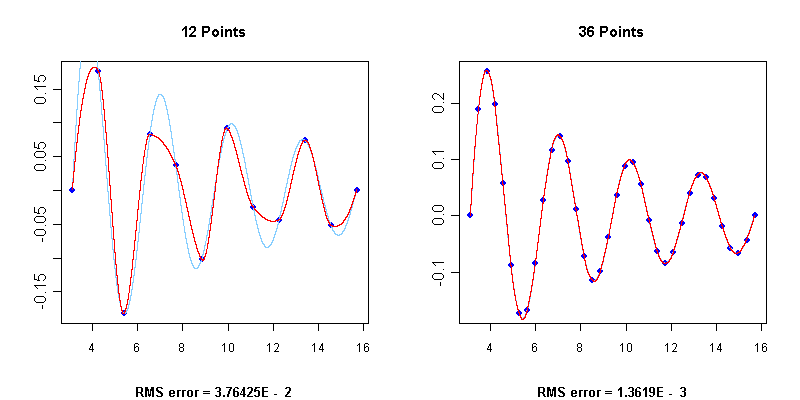
While the first case, with 12 initial points may be a bad fit to the original signal, this fitting illustrates just how carefully the Akima method tries to avoid overshoot. So in many situation where you have a corse set of data points, the Akima method may provide the best fit. Its important to be aware of the nature of the data you analyzing and how likely sudden changes are.

References

• Hiroshi Akima, "A Method of Bivariate Interpolation and Smooth Surface Fitting for Irregularly Distributed Data Points", ACM Transactions on Mathematical Software, Vol. 4, No. 2, June 1978, pp. 148-159. Copyright 1978, Association for Computing Machinery, Inc., reprinted by permission.
• F.R. Ruckdeschel, "BASIC Scientific Subroutines, Vol. II, BYTE/McGRAWW-HILL, 1981.
• For a general overview of different approaches see: http://www.kxcad.net/CINEMA_4D/help/US/html/OSPLINEFORMULA-ID_OBJECTPROPERTIES.html

#include <codecogs/maths/approximation/interpolation/akima.h>

#include <math.h>
#include <iostream>
#include <iomanip>
using namespace std;

#define PI  3.1415
#define N   12

int main()  
{
    // Declare and initialize two arrays to hold the coordinates of the initial data points
    double x[N], y[N];

    // Generate the points
    double xx = PI, step = 4 * PI / (N - 1);
    for (int i = 0; i < N; ++i, xx += step) {
        x[i] = xx;
        y[i] = sin(2 * xx) / xx;
    }

    // Initialize the Akima spline interpolation routine with known data points
    Maths::Interpolation::Akima A(N, x, y);

    // Interrogate spline curve to find interpolated values
    int N_out = 20;
    xx = PI, step = (3 * PI) / (N_out - 1);
    for (int i = 0; i < N_out; ++i, xx += step) {
        cout << "x = " << setw(7) << xx << "  y = ";
        cout << setw(13) << A.getValue(xx) << endl;
	}
    return 0;
}

x =  3.1415  y = -5.89868e-005
x = 3.63753  y =      0.140177
x = 4.13355  y =      0.181798
x = 4.62958  y =     0.0850367
x = 5.12561  y =     -0.129668
x = 5.62163  y =     -0.157484
x = 6.11766  y =   -0.00477961
x = 6.61368  y =     0.0819989
x = 7.10971  y =     0.0712833
x = 7.60574  y =     0.0445423
x = 8.10176  y =   -0.00985429
x = 8.59779  y =    -0.0801354
x = 9.09382  y =     -0.087151
x = 9.58984  y =     0.0367525
x = 10.0859  y =      0.086111
x = 10.5819  y =     0.0312046
x = 11.0779  y =    -0.0221298
x = 11.5739  y =      -0.04029
x =   12.07  y =    -0.0462165
x =  12.566  y =    -0.0233795

See Also

Also consider the regression methods: Discrete, Forsythe, Orthogonal, Stiefel