CodeCogs

Approximates a discrete function using least squares polynomial fitting.

You're viewing an older version of this page (#367). View the current version.

View versions (2)

Interface

#include <codecogs/maths/approximation/regression/discrete.h>

using namespace Maths::Approximation::Regression;

Discrete(int n, double *x, double *y, int degree)
~Discrete()
double getValue(double x)
double getCoefficent(int i)
double IntPower(double x,int k)
double Discrete_once(int N, double *x, double *y, int degree, double a )

Overview

This class approximates an arbitrary discrete function using polynomial least squares fitting.

The algorithm finds the coefficients $a_i$ , with $0 \leq i \leq n$ such that the following polynomial fits the given set of points with minimum error, using leasts squares minimization

$y = a_0 + a_1x + a_2x^2 + \ldots + a_kx^k$

(1)

For this function the residual (or error between y and that calculationed using the coefficients) is given by

$R^2 = \sum_{i=1}^{n} \left [ y_i - (a_0 + a_1 x_i + a_2 x_i^2 + \ldots + a_k x_i^k) \right ]^2$

(2)

From which the rate of change of this error with respect to each constant are, which ideally we want to make zero:

$\frac{\partial(R^2)}{\partial a_0} = -2 \sum_{i=1}^n \left [ y_i - (a_0 + a_1 x_i + a_2 x_i^2 + \ldots + a_k x_i^k) \right ] = 0$

(3)

$\frac{\partial(R^2)}{\partial a_1} = -2 \sum_{i=1}^n \left [ y_i - (a_0 + a_1 x_i + a_2 x_i^2 + \ldots + a_k x_i^k) \right ] x_i = 0$

(4)

$\frac{\partial(R^2)}{\partial a_k} = -2 \sum_{i=1}^n \left [ y_i - (a_0 + a_1 x_i + a_2 x_i^2 + \ldots + a_k x_i^k) \right ] x_i^k = 0$

(5)

Equating to zero and rearranging to seperate the constants a from y, gives:

$a_o n + a_1 \sum_{i=1}^n x_i + \ldots + a_k \sum_{i=1}^n x_i^k = \sum_{i=1}^n y_i$

(6)

$a_o \sum_{i=1}^n x_i + a_1 \sum_{i=1}^n x_i^2 + \ldots + a_k \sum_{i=1}^n x_i^{k+1} = \sum_{i=1}^n x_i y_i$

(7)

$a_o \sum_{i=1}^n x_i^k + a_1 \sum_{i=1}^n x_i^{k+1} + \ldots + a_k \sum_{i=1}^n x_i^{2k} = \sum_{i=1}^n x_i^k y_i$

(8)

which in matrix form, yields

$\left [ \begin{array}{ccccccc} n && \sum_{i=1}^n x_i && \ldots && \sum_{i=1}^n x_i^k \\ \sum_{i=1}^n x_i && \sum_{i=1}^n x_i^2 && \ldots && \sum_{i=1}^n x_i^{k+1} \\ \vdots && \vdots && \ddots && \vdots \\ \sum_{i=1}^n x_i^k && \sum_{i=1}^n x_i^{k+1} && \ldots && \sum_{i=1}^n x_i^{2k} \end{array} \right ] \left [ \begin{array}{c} a_0 \\ a_1 \\ \vdots \\ a_k \end{array} \right ] = \left [ \begin{array}{c} \sum_{i=1}^n y_i \\ \sum_{i=1}^n x_i y_i \\ \vdots \\ \sum_{i=1}^n x_i^k y \end{array} \right ]$

(9)

Solving this solutions using a matrix transpose, yields the coefficients a in terms of x and y.

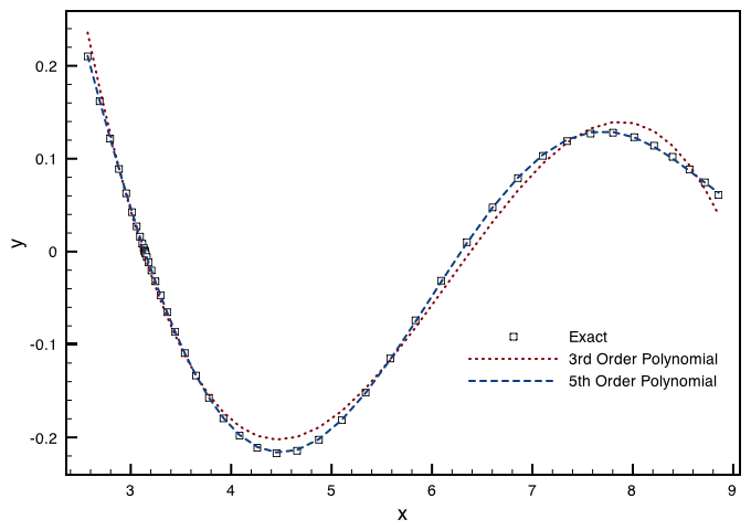
Below you will find the regression graph for a set of points obtained by evaluating the function $f(x) = \sin(x) / x$ . The regression polynomial using a variety of orders are displayed (same results are shown in example below)

References

Mathworld, http://mathworld.wolfram.com/LeastSquaresFittingPolynomial.html

Example 1

The following example displays 10 approximated values (you may change this amount through the N_out variable) for the function $g(x) = \sin(x) / x$ with abscissas equally spaced in the $[ \pi/2, 4\pi]$ interval. The X and Y coordinate arrays are initialized by evaluating this function for N = 20 points equally spaced in the domain from $\pi/2$ to $4\pi$ .

#include <codecogs/maths/approximation/regression/discrete.h>

#include <cmath>
#include <stdio.h>
using namespace std;

#define PI  3.1415926535897932384626433832795
#define N   30

int main() 
{
  // Delvare two arrays to hold the coordinates of initial data points
  double x[N], y[N];
		
  // Generate the points
  double xx = PI/2;
  double step = 2 * PI / (N - 1);
	
  for (int i = 0; i < N; ++i, xx += step) 
  {
    double x2=xx+sin(xx);   // vary x spacing
    x[i] = x2;
    y[i] = sin(x2)/x2;
  }
		
  // Initialize the regression approximation routine with known data points
  Maths::Regression::Discrete A(N, x, y, 3);
  Maths::Regression::Discrete B(N, x, y, 5);
  Maths::Regression::Discrete C(N, x, y, 10);
		
  // Interrogate the regression function to find approximated values
  int N_out =50;
  xx = PI/2 ;
  step = 2 * PI / (N_out - 1);
		
  printf("\nx, exact, discrete_3,  discrete_5,  discrete_10");
		
  for (int i = 0; i < N_out; ++i, xx += step)
  {	
    double x2=xx+sin(xx);
    printf("\n%.4lf, %.6lf, %.6lf, %.6lf, %.6lf", x2, sin(x2)/x2, A.getValue(x2), B.getValue(x2), C.getValue(x2));
  }
  return 0;
}

Output (first 10 numbers):

x, exact, discrete_3,  discrete_5,  discrete_10
2.5708, 0.210169, 0.235747, 0.210570, 0.210190
2.6908, 0.161909, 0.175569, 0.162336, 0.161899
2.7945, 0.121709, 0.127760, 0.122034, 0.121692
2.8824, 0.088920, 0.090229, 0.089115, 0.088905
2.9550, 0.062769, 0.061196, 0.062848, 0.062759
3.0134, 0.042441, 0.039160, 0.042431, 0.042435
3.0585, 0.027131, 0.022864, 0.027058, 0.027128
3.0919, 0.016071, 0.011248, 0.015955, 0.016070
3.1150, 0.008531, 0.003406, 0.008388, 0.008532
3.1296, 0.003821, -0.001463, 0.003663, 0.003822

Members of Discrete

CLASS METHOD

Discrete

Initializes the necessary data for following evaluations of the polynomial.

Parameters

degree

The number of coefficient to be used in the polynomial fitting.

An array [0 to n-1] with y-coordinates of points.

An array [0 to n-1] with x-coordinates of points.

Total number of data points to analyse.

CLASS METHOD

Discrete

Detailed Description...

CLASS METHOD

getValue

Returns the approximated ordinate at the given abscissa.

Parameters

The abscissa of the approximation point

CLASS METHOD

getCoefficent

Returns individual coefficient from the computed polynomial, i.e. $a_i$ in the following equation:

$P(x) = a_0 + a_1x + a_2x^2 + \ldots + a_nx^n$

(10)

Example 1

...
Maths::Regression::Discrete A(N, x, y, 7); 
for(int i=0;i<7;i++) printf("\n coefficient %d is %lf", A.getCoefficient(i)); 
...

Parameters

The ith coefficient, starting at i=0 to degree.

CLASS METHOD

IntPower

CLASS METHOD

Discrete_once

This function implements the Discrete class for one off calculations, thereby avoid the need to instantiate the Discrete class yourself.

Example 1

The following graph is constructed from interpolating the following values:

x = 1  y = 0.22
x = 2  y = 0.04
x = 3  y = -0.13
x = 4  y = -0.17
x = 5  y = -0.04
x = 6  y = 0.09
x = 7  y = 0.11

\graph N=7 x="1 2 3 4 5 6 7" y="0.22 0.04 -0.13 -0.17 -0.04 0.09 0.11" a=1:7 degree=5 .input

Parameters

The number of initial points

The x-coordinates for the initial points

The y-coordinates for the initial points

degree

The number of coefficient to be used in the polynomial fitting (the order)

the x-coordinate for the point to be computed

Returns

the y-coordinate that corresponds to a.