
Logistic
Evaluates the logistic regression curve built from a given set of points.
You're viewing an older version of this page (#92). View the current version.
Interface
#include <codecogs/maths/approximation/regression/logistic.h>
using namespace Maths::Approximation::Regression;
Overview
The logit of a number is
The logit function is the inverse of the sigmoid, or logistic function. If is a probability then
is the corresponding odds, and the logit of the probability is the logarithm of the odds; similarly the difference between the logits of two probabilities is the logarithm of the odds-ratio, thus providing an additive mechanism for combining odds-ratios.
Logits are used for various purposes by statisticians. In particular there is the "logit model" of which the simplest sort is
where is some quantity on which success or failure in the
-th in a sequence of Bernoulli trials may depend, and
is the probability of success in the
-th case. For example,
may be the age of a patient admitted to a hospital with a heart attack, and "success" may be the event that the patient dies before leaving the hospital (another instance of the reason why the words "success" and "failure" in speaking of Bernoulli trials should be taken with large doses of salt). Having observed the values of
in a sequence of cases and whether there was a "success" or a "failure" in each such case, a statistician will often estimate the values of the coefficients
and
by the method of maximum likelihood. The result can then be used to assess the probability of "success" in a subsequent case in which the value of
is known. Estimation and prediction by this method are called <em> logistic regression </em>.
As you may have noticed there is a link between the logistic and the linear regression methods, through the function. In other words,
Applying the exponential in both sides of the equality and doing further calculations, we arrive at the following relation
where and
are the parameters of the associated linear regression, intercept and slope.
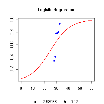
Below you will find the regression graph for a set of arbitrary points, coloured in blue. The regression curve, displayed in red, has been calculated using this class.
Example 1
The following example evaluates the logistic curve for a given set of points, which is also displayed in the previous graph. The abscissas are equally spaced in the interval [10, 50] with a step of 5.
#include <codecogs/maths/regression/logistic.h>
#include <iostream>
#include <iomanip>
using namespace std;

int main() {
    double x[6] = {   28,    29,    30,    31,    32,    33};
    double y[6] = {.3333, .4000, .7778, .7778, .8000, .9333};

    Maths::Regression::Logistic A(6, x, y);

    cout << "Logistic regression values" << endl << endl;
    for (int i = 10; i <= 50; i += 5) {
        cout << "x = " << setw(3) << i << "  y = " << A.getValue(i);
        cout << endl;
	}
    return 0;
}
Output:
Logistic regression values

x =  10  y = 0.143118
x =  15  y = 0.233325
x =  20  y = 0.356719
x =  25  y = 0.502592
x =  30  y = 0.648024
x =  35  y = 0.770364
x =  40  y = 0.859406
x =  45  y = 0.917614
x =  50  y = 0.95304
References
Members of Logistic
CLASS METHOD
Logistic
Initializes the class by calculating the slope and intercept of the corresponding linear regression function.
Parameters
CLASS METHOD
Logistic
Class destructor (empty)
CLASS METHOD
getValue
CLASS METHOD
Logistic_once
This function implements the Logistic class for one off calculations, thereby avoid the need to instantiate the Logistic class yourself.
Example 1
The following graphs fits a single regression curve to the following values:
x = 23.2  y = 0.02
x = 33.3  y = 0.04
x = 33.5  y = 0.13
x = 34   y = 0.17
x = 34.2  y = 0.18
x = 34.2  y = 0.15
x = 34.4  y = 0.11
\graph n=7 x="23.2 33.3 33.5 34 34.2 34.2 34.4" y="0.02 0.04 0.13 0.17 0.18 0.15 0.11" a=0:150 .input