
Orthogonal
Approximates an arbitrary function using orthogonal polynomials.
You're viewing an older version of this page (#93). View the current version.
Interface
#include <codecogs/maths/approximation/regression/orthogonal.h>
using namespace Maths::Approximation::Regression;
Overview
This class approximates an arbitrary discrete function by least squares fitting orthogonal polynomials. In mathematics, two polynomials f and g are orthogonal to each other with respect to a nonnegative <em> weight function </em> w precisely if
In other words, if polynomials are treated as vectors and the inner product of two polynomials and
is defined as
then the orthogonal polynomials are simply orthogonal vectors in this inner product space. The algorithm uses this class of polynomials to achieve the best curve fitting by minimization in terms of least squares.
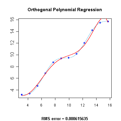
Below you will find the regression graph for a set of points obtained by evaluating the function , displayed in light blue, at particular abscissas. The regression polynomial, displayed in red, has been calculated using this class. The root mean squared error is also displayed.
References
- Jean-Pierre Moreau's Home Page, http://perso.wanadoo.fr/jean-pierre.moreau/
- Tuan Dang Trong, "Numath Library" in Fortran 77
Example 1
The following example displays 10 approximated values (you may change this amount through the N_out variable) for the given function with abscissas equally spaced in the
interval. The X and Y coordinate arrays are initialized by evaluating this function for N = 12 points equally spaced in the domain from
to
.
#include <codecogs/maths/regression/orthogonal.h>

#include <cmath>
#include <iostream>
#include <iomanip>
using namespace std;

#define PI  3.1415926535897932384626433832795
#define N   12

int main()
{
    // Declare and initialize two arrays to hold the coordinates of the initial data points
    double x[N], y[N];

    // Generate the points
    double xx = PI, step = 4 * PI / (N - 1);
    for (int i = 0; i < N; ++i, xx += step) {
        x[i] = xx;
        y[i] = sin(xx) + xx;
    }

    // Initialize the regression approximation routine with known data points
    Maths::Regression::Orthogonal A(N, x, y, 12);

    // Interrogate the regression function to find approximated values
    int N_out = 10;
    xx = PI, step = (3 * PI) / (N_out - 1);
    for (int i = 0; i < N_out; ++i, xx += step) {
        cout << "x = " << setw(7) << xx << "  y = ";
        cout << setw(11) << A.getValue(xx) << endl;
	}
    return 0;
}
Output:
x = 3.14159  y =     3.14159
x = 4.18879  y =     3.32247
x = 5.23599  y =     4.37014
x = 6.28319  y =     6.28307
x = 7.33038  y =     8.19649
x = 8.37758  y =     9.24353
x = 9.42478  y =     9.42486
x =  10.472  y =     9.60584
x = 11.5192  y =     10.6533
x = 12.5664 y = 12.566Members of Orthogonal
CLASS METHOD
Orthogonal
Initializes the necessary data for following evaluations of the polynomial.
Parameters
CLASS METHOD
Orthogonal
Class destructor
CLASS METHOD
getValue
Returns the approximated ordinate at the given abscissa.
Parameters
STATIC CLASS METHOD
prod
CLASS METHOD
Orthogonal_once
This function implements the Orthogonal class for one off calculations, thereby avoid the need to instantiate the Orthogonal class yourself.
Example 1
The following graphs are constructed from the interpolation of the following values, using a 3rd order polynomial and then 8th order polynomial, respectively:
x = 1  y = 0.22
x = 2  y = 0.04
x = 3  y = -0.13
x = 4  y = -0.17
x = 5  y = -0.04
x = 6  y = 0.09
x = 7  y = 0.11
\graph n=7 x="1 2 3 4 5 6 7" y="0.22 0.04 -0.13 -0.17 -0.04 0.09 0.11" degree=3 a=1:7 \graph n=7 x="1 2 3 4 5 6 7" y="0.22 0.04 -0.13 -0.17 -0.04 0.09 0.11" degree=6 a=1:7