
Thermodynamic Cycles
Key facts The thermal efficiency of any engine working between the temperatures of T\_1 and T\_2 is:
with the equality being satisfied only for the Carnot efficiency. Therefore, the Carnot cycle is the cycle with the highest possible thermal efficiency, while in order to increase the efficiency of all the other engines the (T\_2-T\_1) value should be increased.
An introduction to thermodynamic cycles, also discussing the Carnot cycle
You're viewing an older version of this page (#3630). View the current version.
The thermodynamic cycle consists of a series of operations (e.g. expansion/compression of a volume - see Figure 1) carried out on a gas or steam (which is often called a working substance, WS), after which it returns to its original state.
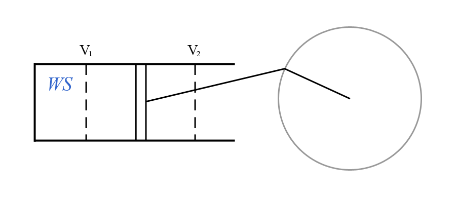
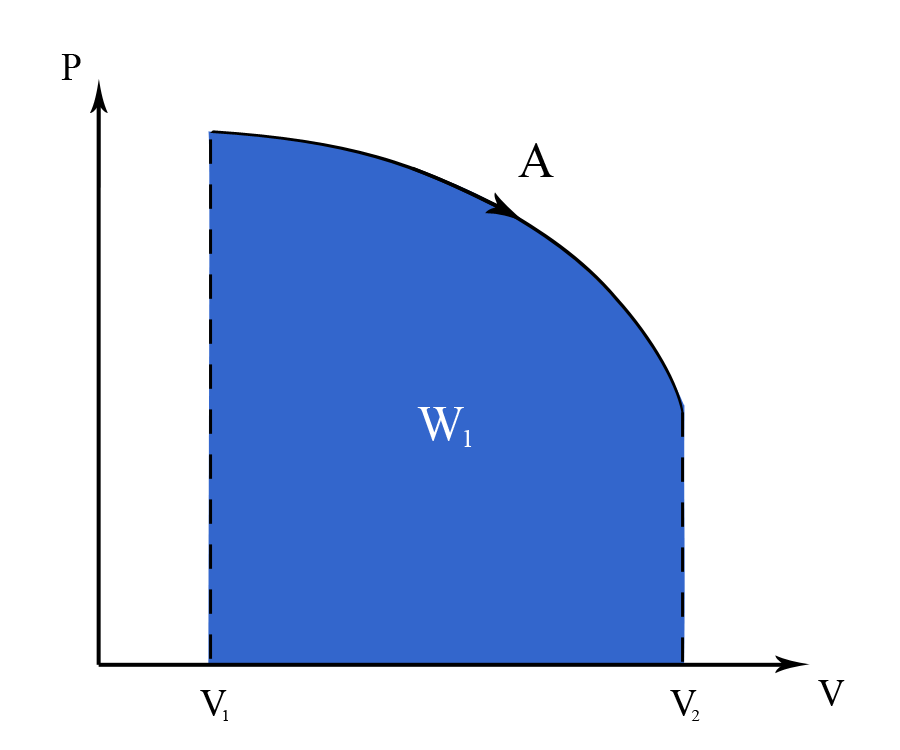
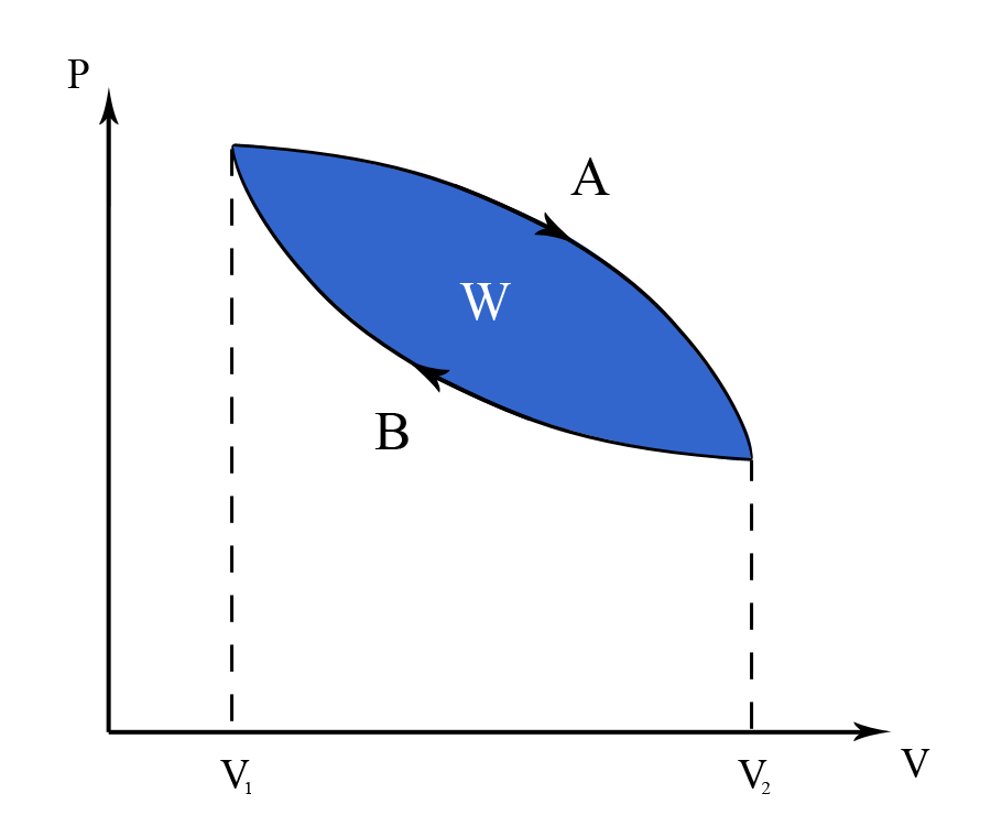
For example, imagine that initially there is an expansion of volume from V\_1 to V\_2, corresponding to a work output of W\_1. Figure 2 shows such a process with a pressure (P) - volume (V) plot, where the work output (W\_1) equals the area under curve A 9 (shaded blue).
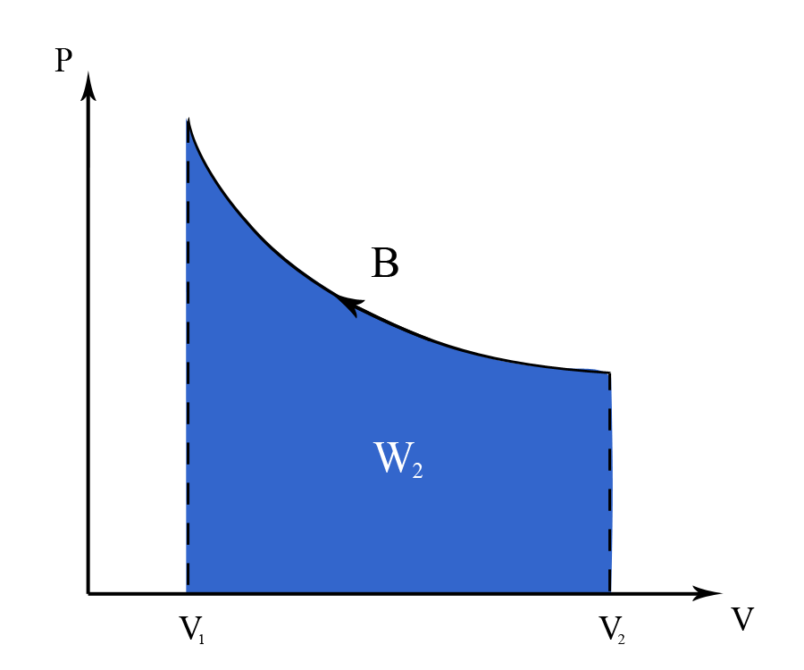
Next the gas is compressed back to its original volume, i.e. V\_2 back to V\_1, which requires a work input of W\_2 (the shaded area under the curve in Figure 3).
When we combine the two processes on a single plot, we get a closed loop (see Figure 4A). This closed loop corresponds to a thermodynamic cycle.
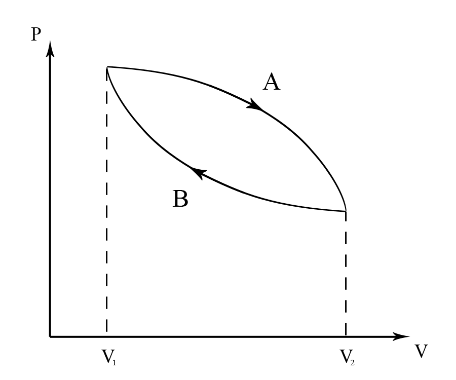
As the net work output is given by:
it will thus equal the area of the cycle (the blue shaded area in Figure 4B).
Such thermodynamic cycles can also be represented on temperature () - entropy (
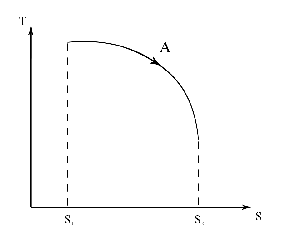
) diagrams. For example, imagine that initially there is a certain amount of heat supplied (
) to the WS, leading to an increase in entropy. If we are to illustrate such a process on a
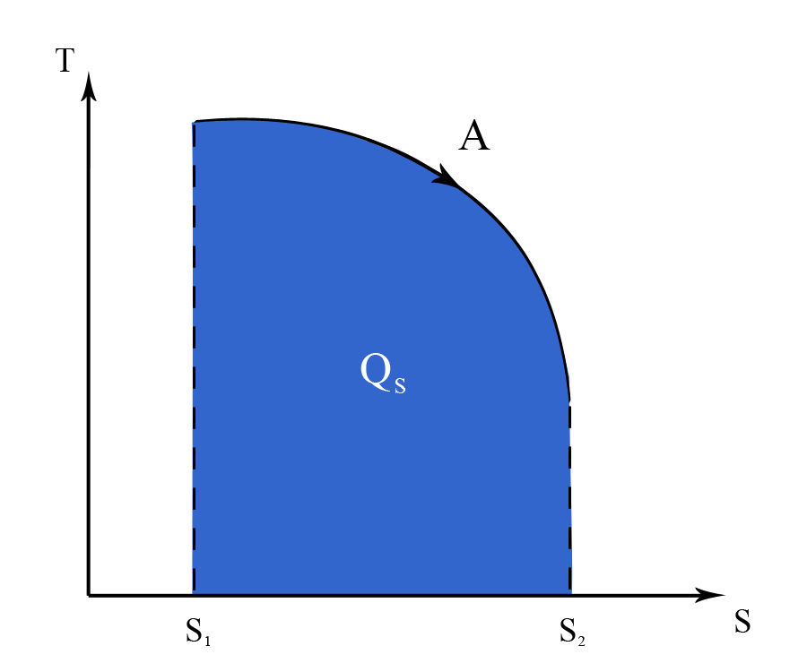
plot (see Figure 5A), then the heat energy supplied
will equal the area under curve
(the blue shaded area in Figure 5B).
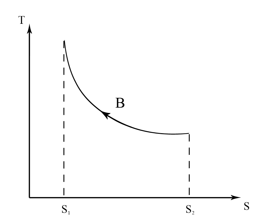
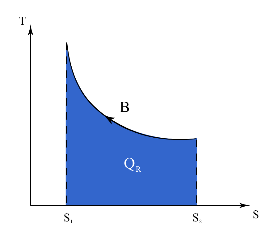
Next, consider that there is a certain amount of heat rejected in the WS and in losses (), reverting the system back to its initial state. By plotting this process on a
diagram (see Figure 6A), the heat rejected
will equal the area under curve
(the blue shaded area in Figure 6B).
If we are to illustrate both processes on a single plot, then we will get again a closed loop, corresponding to the thermodynamic cycle (see Figure 7A)
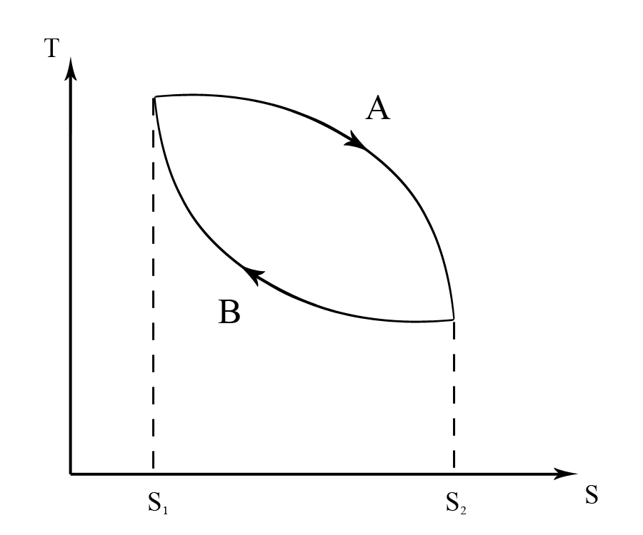
By denoting the energy of the WS at the start of the cycle with , and the energy of the WS at the end of the cycle with
, and by applying the law of conservation of energy, we can write that:
where is the work output (for a more detailed discussion on the law of conservation of energy see First Law of Thermodynamics ).
However, as (the system is reverted back to its initial state), equation (#2) becomes:
from which:
Therefore, when plotting the thermodynamic cycle on a diagram (as in Figure 7A), the work output will again equal the area of the cycle (the blue shaded area in Figure 7B).
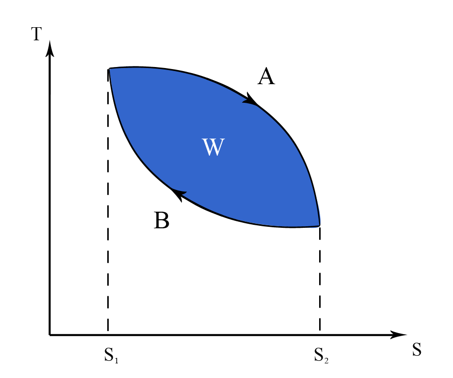
It is important to note that, although the work done can be calculated from the area of the thermodynamic cycle for both a and a
plot, the results obtained are expressed in different units. For example, if calculating in imperial units, the area of the cycle on the
diagram gives the work done in
, while the area of the cycle on the
diagram gives the work done in
.