Univariate Regression

A function expresses the idea that one quantity (the argument of the function) completely determines another quantity (the value).

A polynomial is an expression of finite length constructed from variables and constants, using only the operations of addition, subtraction, multiplication, and non-negative integer exponents.

univariate regression, polynomial regression, orthogonal polynomials, nonlinear

You're viewing an older version of this page (#3681). View the current version.

View versions (2)

Univariate regression is an area of curve-fitting which, given a function $f$ depending on some parameters, finds the parameters such that $f$ provides the best fit to a series of two-dimensional data points, in a certain sense. It is called univariate as the data points are supposed to be sampled from a one-variable function. Compare this to multivariate regression, which aims at fitting data points sampled from a function of several variables.

Formally speaking, consider a series of $N$ data points $(x_1, y_1), (x_2, y_2), \ldots, (x_N, y_N)$ and, for the sake of simplicity, consider that $x_1 < x_2 < \ldots < x_N$ , i.e. the points are distinct and are in increasing order with respect to $x$ . By doing least squares fitting on these data points we mean finding the parameters $\alpha_1, \alpha_2, \ldots, \alpha_k$ of a function $f_{\displaystyle \alpha_1, \alpha_2, \ldots, \alpha_k} : [x_1, x_n] \to \mathbb{R}$ such that the sum of squared residuals

$\sum_{i = 1}^N \left[f_{\displaystyle \alpha_1, \alpha_2, \ldots, \alpha_k}(x_i) - y_i\right]^2$

is minimized. Provided that $f$ depends linearly on its parameters, the method is called linear regression, otherwise it is called nonlinear regression. For example, straight line regression, parabolic regression and polynomial regression are all linear regression models since the function $f$ is of the form

$f_{\displaystyle \alpha_0, \alpha_1, \ldots, \alpha_k}(x) = \alpha_0 + \alpha_1 x + \alpha_2 x^2 + \ldots + \alpha_k x^k,$

which clearly depends linearly on its parameters. As opposed to this, logistic regression, for example, is a nonlinear regression model since the fitting function is of the form

$f_{\displaystyle \alpha_1, \alpha_2}(x) = \frac{1}{1 + e^{\displaystyle -\alpha_1 - \alpha_2 x}}$

which is a nonlinear function of $\alpha_1$ and $\alpha_2$ .

In the following, let us consider each case and briefly explain how the corresponding optimal parameters can be derived.

Polynomial regression

One linear regression method is that of polynomial regression, which refers to finding the polynomial function that provides the least squares fitting to a series of data points.

More precisely, if the polynomial function $f$ of degree $k$ is given by :

$f_{\displaystyle \alpha_0, \alpha_1, \ldots, \alpha_k}(x) = \alpha_0 + \alpha_1 x + \alpha_2 x^2 + \ldots + \alpha_k x^k,$

then the optimal parameters $\alpha_0, \alpha_1, \ldots, \alpha_k$ can be found by solving the following system of linear equations:

$\left [ \begin{array}{lllllll} N & & \sum_{i=1}^N x_i && \ldots & & \sum_{i=1}^N x_i^k \\ \\ \sum_{i=1}^N x_i & & \sum_{i=1}^N x_i^2 && \ldots & & \sum_{i=1}^N x_i^{k+1} \\ \\ \vdots & & \vdots & & \ddots & & \vdots \\ \\ \sum_{i=1}^N x_i^k & & \sum_{i=1}^N x_i^{k+1} & & \ldots & & \sum_{i=1}^N x_i^{2k} \end{array} \right] \left[ \begin{array}{l} \alpha_0\\ \\ \alpha_1\\ \\ \vdots\\ \\ \alpha_k \end{array} \right] = \left [ \begin{array}{l} \sum_{i=1}^N y_i\\ \\ \sum_{i=1}^N x_i y_i\\ \\ \vdots\\ \\ \sum_{i=1}^N x_i^k y_i \end{array} \right]$

For $k = 1$ , the function $f$ only depends on two parameters

$f_{\displaystyle \alpha_0, \alpha_1}(x) = \alpha_0 + \alpha_1 x$

and, in this case, the method is called straight line regression. The previous linear system becomes

$\left[ \begin{array}{lll} N & & \sum_{i=1}^N x_i \\ \\ \sum_{i=1}^N x_i & & \sum_{i=1}^N x_i^2 \end{array} \right] \left[ \begin{array}{l} \alpha_0 \\ \\ \alpha_1 \end{array} \right] = \left[ \begin{array}{l} \sum_{i=1}^N y_i\\ \\ \sum_{i=1}^N x_i y_i \end{array} \right]$

which gives the optimal parameters (as its solution)

$\alpha_1 = \frac{\sum_{i=1}^N (x_i - \overline{x})(y_i - \overline{y})}{\sum_{i=1}^N (x_i - \overline{x})}, \qquad \alpha_0 = \overline{y} - \alpha_1 \overline{x},$

where $\overline{x}$ and $\overline{y}$ are the averages:

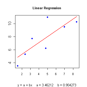
$\overline{x} := \frac{1}{N} \sum_{i=1}^N x_i, \qquad \overline{y} := \frac{1}{N} \sum_{i=1}^N y_i.$

For example, consider the set of 7 points:

$(1.5, 3.5),\ (2.4, 5.3),\ (3.2, 7.7),\ (4.8, 6.2),\ (5, 11),\ (7, 9.5),\ (8.43, 10.27)$

Then the optimal values of the parameters are

$\alpha_0 = 3.46212, \quad \alpha_1 = 0.904273,$

which gives the fitting line $f(x) = 3.46212 + 0.904273\ x$ . The following graph shows the data points and the regression line.

Straight line regression is also implemented as the component Linear.

The optimal parameters for the case $k = 2$ can be found in a similar manner. Instead of going into further technical details, let us look at the following graph which shows the quadratic regression polynomial in red for the series of data points shown in blue, sampled from a sine-like function.

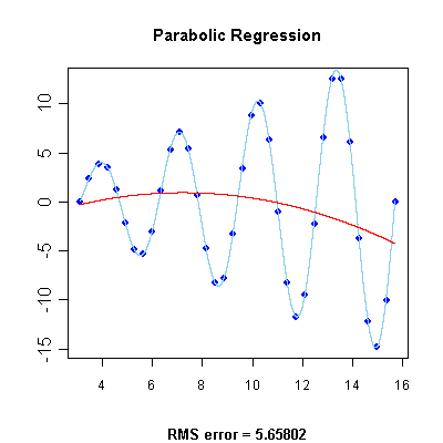
Notice that the resulting fitting curve looks more like a parabola and this is due to the fact that we may have chosen the wrong family of functions to provide the fit (polynomial ones), or perhaps the degree of the regression polynomial is too small. Parabolic regression is available as Parabolic.

For the general case of regression polynomials of arbitrary degree, the component Discrete is available.

Orthogonal polynomial regression

Orthogonal polynomial regression is an extension of polynomial regression, in the sense that instead of using $x^0, x^1, x^2, \ldots, x^k$ as the factors in the fitting function $f$ , some special kind of functions $\phi_0(x), \phi_1(x), \ldots, \phi_k(x)$ are used and thus the expression for $f$ becomes:

$f_{\displaystyle \alpha_0, \alpha_1, \ldots, \alpha_k}(x) = \alpha_0 \phi_0(x) + \alpha_1 \phi_1(x) + \ldots + \alpha_k \phi_k(x).$ More precisely, the functions $\phi_0, \phi_1, \ldots\$ should be polynomial, listed in increasing order of their degree and also with the property that

$\int_{x_1}^{x_n} \phi_i(x) \phi_j(x) w(x)\ {\rm d}x = 0.$

for any $i \neq j$ , where $w : [x_1, x_n] \to \mathbb{R}$ is some weight function. In other words, the sequence of polynomial functions $\phi_0, \phi_1, \ldots\$ is orthogonal.

Apart from this, the regression using orthogonal polynomials uses the same idea of minimizing the sum of squared residuals. It is also implemented as the component Orthogonal.

Below is a graph of a series of data points, shown in blue, and their corresponding fitting function, determined by the method of orthogonal polynomial regression.

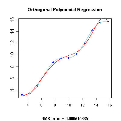
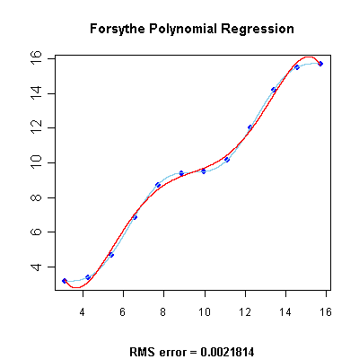
We may as well use certain types of orthogonal polynomials, instead of general ones as in the above method. For instance, we can use the Forsythe orthogonal polynomials, leading to the method of Forsythe polynomial regression, available as Forsythe.

In the image below, we have used Forsythe regression on the same series of data points as in the previous graph.

Nonlinear regression

As mentioned at the beginning of this reference page, nonlinear regression refers to the cases when the fitting function depends nonlinearly on its parameters. Therefore $f$ can virtually be any function with this property. Depending on the experiment from which the data points were obtained and the statistical properties of the phenomenon which took place, we may choose between various families of nonlinear regression functions.

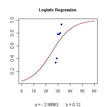
To name a few nonlinear regression models, logistic regression is given by the fitting function

$f_{\displaystyle \alpha_1, \alpha_2}(x) = \frac{1}{1 + e^{\displaystyle -\alpha_1 - \alpha_2 x}}$

and is also implemented as Logistic. In the following image you can see the logistic regression curve in red, for the series of data points shown in blue.

Other nonlinear regression models include the Gompertz model, given by the fitting function

$f_{\displaystyle \alpha_1, \alpha_2, \alpha_3}(x) = \alpha_1 e^{\displaystyle -e^{-\alpha_2 - \alpha_3 x}},$

or Richard's model, given by:

$f_{\displaystyle \alpha_1, \alpha_2, \alpha_3, \alpha_4}(x) = \frac{\alpha_1}{\left[1 + e^{\displaystyle -\alpha_2 - \alpha_3 x}\right]^{\alpha_4}}.$

Author

Lucian Bentea (September 2008)

References

Franklin A. Graybill, Hariharan K. Iyer, Regression Analysis. Concepts and Applications, Duxbury Press, Belmont, California.
http://en.wikipedia.org/wiki/Curve_fitting
http://en.wikipedia.org/wiki/Regression_analysis
http://en.wikipedia.org/wiki/Least_squares
http://en.wikipedia.org/wiki/Orthogonal_polynomials