
Velocity and Acceleration of a Piston
Key facts
For a piston with the crank radius , the rod length
, the crank angle
, and the crank angular velocity
, its velocity can be written as:
and its acceleration:
where .
An analysis of the velocity and acceleration of a piston
You're viewing an older version of this page (#3610). View the current version.
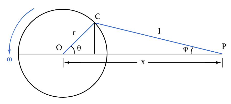
In order to define the velocity and acceleration of a piston, consider the mechanism in Figure 1, where the crank is driven with the uniform angular velocity
. Also, let
be the crank radius,
the rod length,
the position of the piston pin from the crank center,
the
angle, and
the
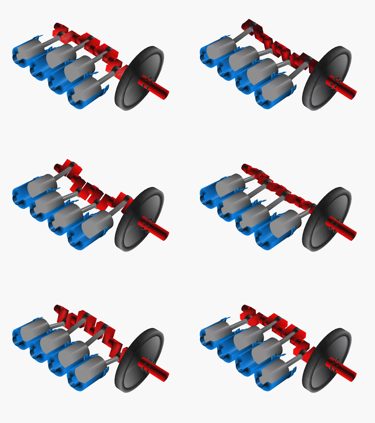
angle (the crank angle). Such a mechanism in motion can be seen in Figure 2, where the crankshaft is depicted with red, and the pistons with gray (to see the animation click on the thumbnail).
From Figure 1 it can be seen that:
It can also be noted from Figure 1 that:
Squaring equation (#2) gives:
which can also be written as:
This eventually leads to:
where .
By using this expression of in equation (#1), we obtain:
which can also be written as:
and, furthermore, as:
In order to calculate the piston velocity, we differentiate (#8) with respect to time, when we get:
The piston acceleration can then be calculated by differentiating again with respect to time, when we obtain:
Note that in these equations the positive direction of velocity and acceleration is away from the crankshaft.
In normal situations and
can be neglected in comparison with
, and, thus, the above equations can be reduced to:
Example 1 [imperial]
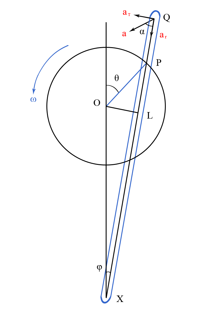
In the crank and slotted lever mechanism diagramed in Figure E1, the crank is driven at a uniform speed of
radians per second. If
is the perpendicular from
on
,
being the center-line of the slotted lever, prove that the angular acceleration of the slotted lever is given by:
Also, find the magnitude and direction of the acceleration of the point when the crank angle is
, given that
,
, and
.
From the diagram we can write that:
from which:
By differentiating (#3) with respect to time, we get:
which leads to:
From Figure E1 we can write that:
Thus, equation (#5) becomes:
or:
By differentiating (#5) with respect to time, we obtain:
By substituting in equation (#10) with the expression from (#9), we can write:
or:
By replacing the numerical values in equation (#3), we can write that:
As:
equation (#13) becomes:
which gives:
Thus, we get that:
and, by using this value, we also obtain that:
Furthermore, by replacing numerical values in (#9) and (#12), we respectively get that:
In order to calculate the acceleration of ,
, we are going to split it in a tangential component,
, perpendicular to
, and a radial component,
, in the direction of
(see Figure E1). Also, let
be the angle which defines the direction of the acceleration. We can write that:
from which we get the magnitude of acceleration:
Also, as:
we obtain the direction of acceleration:
Example 2 [metric]
In the crank and slotted lever mechanism diagramed in Figure E1, the crank is driven at a uniform speed of
radians per second. If
is the perpendicular from
on
,
being the center-line of the slotted lever, prove that the angular acceleration of the slotted lever is given by:
Also, find the magnitude and direction of the acceleration of the point when the crank angle is
, given that
,
, and
.
From the diagram we can write that:
from which:
By differentiating (#3) with respect to time, we get:
which leads to:
From Figure E1 we can write that:
Thus, equation (#5) becomes:
or:
By differentiating (#5) with respect to time, we obtain:
By substituting in equation (#10) with the expression from (#9), we can write:
or:
By replacing the numerical values in equation (#3), we can write that:
As:
equation (#13) becomes:
which gives:
Thus, we get that:
and, by using this value, we also obtain that:
Furthermore, by replacing numerical values in (#9) and (#12), we respectively get that:
In order to calculate the acceleration of ,
, we are going to split it in a tangential component,
, perpendicular to
, and a radial component,
, in the direction of
(see Figure E1). Also, let
be the angle which defines the direction of the acceleration. We can write that:
from which we get the magnitude of acceleration:
Also, as:
we obtain the direction of acceleration: